3.7. 主成分分析(PCA)实战
本文紧承 3.4. 主成分分析(PCA)理论, 没看过的建议先看。
3.7.1. 一些准备工作
接下来,请你确保你的Python环境中有pandas、matplotlib、scikit-learn和numpy这几个包,如果没有,请在终端输入指令以下载和安装:
pip install pandas matplotlib scikit-learn numpy
Iris数据集在scikit-learn中内置有,不需要额外安装。
3.7.2. 读取数据集
Iris数据集内置在sklearn里了,我们可以通过sklearn来引入:
# 加载Iris数据集
from sklearn import datasets
iris = datasets.load_iris()
X = iris.data  # 4维特征
y = iris.target  # 目标分类
Iris数据集在 3.5. 决策树实战 中就讲过,这里我再简单介绍一下:
这个数据集总共会有三种共150条记录,每类各50个数据。每条记录都有4项特征:
- 花萼长度(Sepal Length)
- 花萼宽度(Sepal Width)
- 花瓣长度(Petal Length)
- 花瓣宽度(Petal Width)
我们会通过花萼和花瓣的这4个特征来对花进行分类:
- iris-setosa(在数据集中的标签是0)
- iris-versicolour(在数据集中的标签是1)
- iris-virginica(在数据集中的标签是2)
以下是Iris数据集里的部分数据:
| 花萼长度 | 花萼宽度 | 花瓣长度 | 花瓣宽度 | 属种 |
|---|---|---|---|---|
| 5.1 | 3.5 | 1.4 | 0.2 | setosa |
| 4.9 | 3.0 | 1.4 | 0.2 | setosa |
| 4.7 | 3.2 | 1.3 | 0.2 | setosa |
| 4.6 | 3.1 | 1.5 | 0.2 | setosa |
| 5.0 | 3.6 | 1.4 | 0.2 | setosa |
| 5.4 | 3.9 | 1.7 | 0.4 | setosa |
| 4.6 | 3.4 | 1.4 | 0.3 | setosa |
| 5.0 | 3.4 | 1.5 | 0.2 | setosa |
3.7.3. 数据标准化
我先把主成分分析的所有步骤都粘在这里:
- 原始数据预处理:也就是标准化,因为不同维度的量纲不一定一样。我们先把数据进行一次变换,保证均值$\mu = 0$, 标准差$\sigma = 1$
- 计算协方差矩阵特征向量、及数据在各特征向量投影后的方差
- 按投影方差(特征值)对主成分方向排序:保留方差最大的$k$个方向,丢弃低方差方向(信息较少),最后降到$k$维
- 选取这$k$维特征向量,计算数据在其形成空间的投影
首先就进行标准化,库提供了fit_transform函数来处理:
# 数据标准化
from sklearn.preprocessing import StandardScaler
scaler = StandardScaler()
X_scaled = scaler.fit_transform(X)
3.7.4. 数据降维
然后我们通过:
# 进行PCA降维到2维
from sklearn.decomposition import PCA
pca = PCA(n_components=2)
X_pca = pca.fit_transform(X_scaled)
n_components的值可以控制降维后的维度数量.fit_transform方法可以进行降维
3.7.5. 降维之后的数据可视化
使用matplotlib进行数据可视化:
# 可视化降维后的数据
import matplotlib.pyplot as plt
plt.figure(figsize=(8, 6))
colors = ['red', 'green', 'blue']
labels = iris.target_names
for i in range(len(colors)):
    plt.scatter(X_pca[y == i, 0], X_pca[y == i, 1], color=colors[i], label=labels[i], alpha=0.7, edgecolors='k')

plt.xlabel('Principal Component 1')
plt.ylabel('Principal Component 2')
plt.title('PCA of Iris Dataset')
plt.legend()
plt.grid()
plt.show()
图片输出:
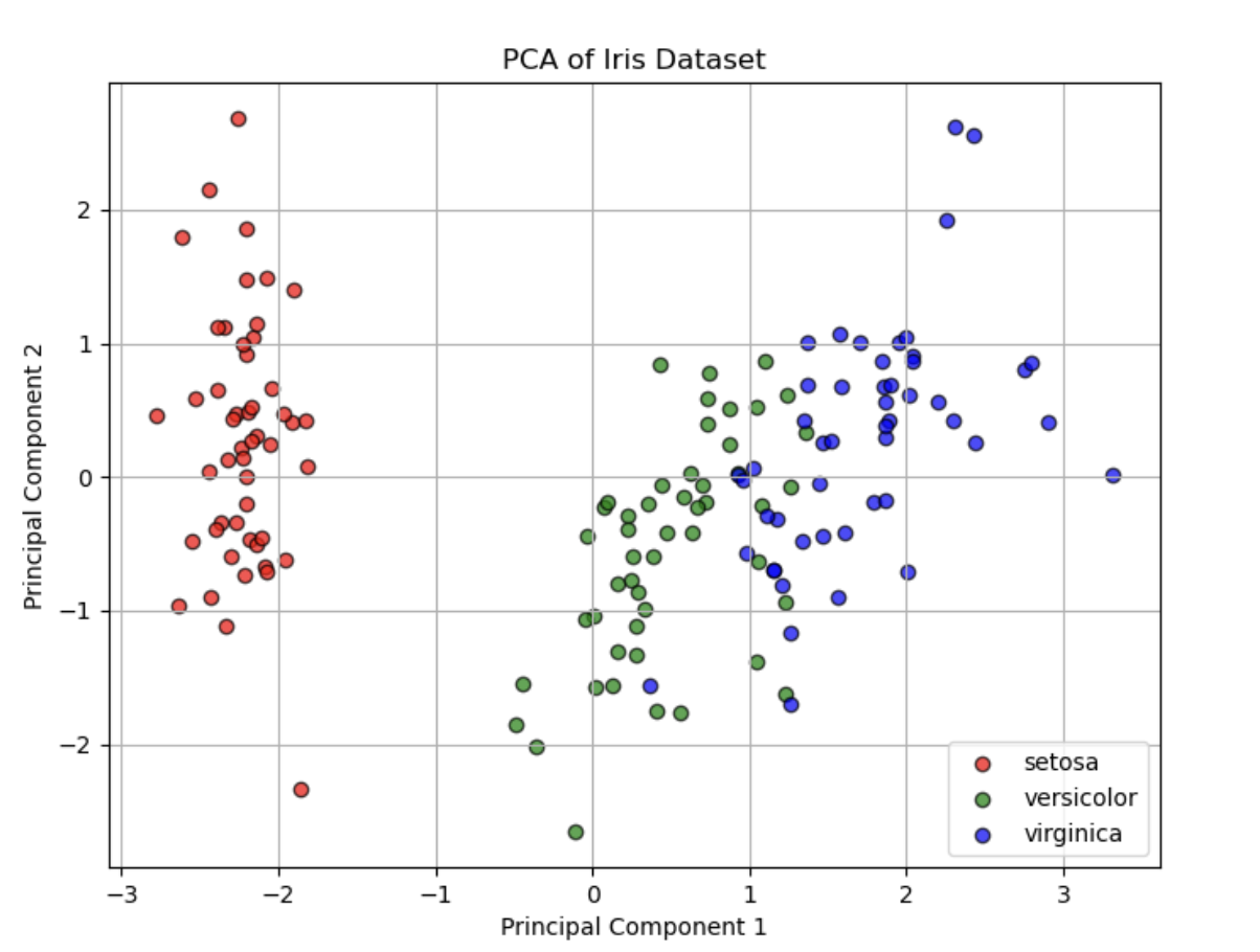
从这幅图中可以看出,降维之后的数据仍保持清晰结构,不同标签的散点还是能够大概分开的。
3.7.6. 组合变量的查看
刚刚表格的两个轴就被替换为了两个组合变量,那我们如何确定是哪两个因子合成了一个轴呢?我们可以查看主成分载荷(Principal Component Loadings),即PCA的特征向量(Components)。这些载荷表示每个原始特征在主成分上的贡献。
在sklearn中,可以使用pca.components_属性获取:
import pandas as pd

# 获取主成分载荷矩阵
loadings = pca.components_

# 创建一个DataFrame,查看每个原始特征在新主成分上的权重
feature_names = iris.feature_names
pc_loadings = pd.DataFrame(loadings, columns=feature_names, index=['PC1', 'PC2'])

print("Principal Component Loadings:")
print(pc_loadings)
输出:
Principal Component Loadings:
     sepal length (cm)  sepal width (cm)  petal length (cm)  petal width (cm)
PC1           0.521066         -0.269347           0.580413          0.564857
PC2           0.377418          0.923296           0.024492          0.066942
- 每一行(PC1, PC2)对应一个主成分
- 每一列(原始特征)表示该特征在主成分上的贡献系数
- 数值的绝对值越大,表示该特征对该主成分的贡献越大
- 正负号表示该特征在该主成分上的方向(正相关或负相关)
据此可以解读出:
- 第一主成分 (PC1)主要由petal length (0.580) 和petal width (0.564) 决定,因为两者对于PC1的贡献最大
- 第二主成分 (PC2)sepal width (0.923) 对 PC2 贡献最大,远高于其他特征。sepal length (0.377) 也有一定贡献,但远不及sepal width。
3.7.7. 降维损失分析
解释方差(Explained Variance)
PCA的每个主成分都保留了数据的一部分方差信息。可以查看解释方差比例(explained variance ratio) 来评估降维损失:
import numpy as np

explained_variance_ratio = pca.explained_variance_ratio_
print("Explained variance ratio:", explained_variance_ratio)
print("Total variance retained:", np.sum(explained_variance_ratio))
explained_variance_ratio_表示每个主成分解释的方差比例np.sum(explained_variance_ratio_)表示保留的总方差比例,越接近 1,说明损失越小
输出:
Explained variance ratio: [0.72962445 0.22850762]
Total variance retained: 0.9581320720000165
重构误差(Reconstruction Error)
PCA进行降维后,可以将数据从低维空间逆变换(inverse_transform) 回原始空间,然后计算均方误差(MSE) 以评估损失:
X_reconstructed = pca.inverse_transform(X_pca)  # 逆变换回原始空间
reconstruction_error = np.mean((X_scaled - X_reconstructed) ** 2)
print("Reconstruction Error (MSE):", reconstruction_error)
- 误差越小,说明降维保留的信息越多
输出:
Reconstruction Error (MSE): 0.0418679279999836