2.4. 卷积神经网络(CNN)实战(进阶):使用VGG-16进行图像特征提取
本文承接 2.2. 卷积神经网络(CNN)模型理论(进阶):图像填充、LeNet、AlexNet,没看过的建议先看前文。
2.4.1. VGG-16的架构
在本文中我们会使用VGG-16进行图像特征提取,然后构建自己的二分类模型,我们先来回顾一下VGG-16模型的架构:
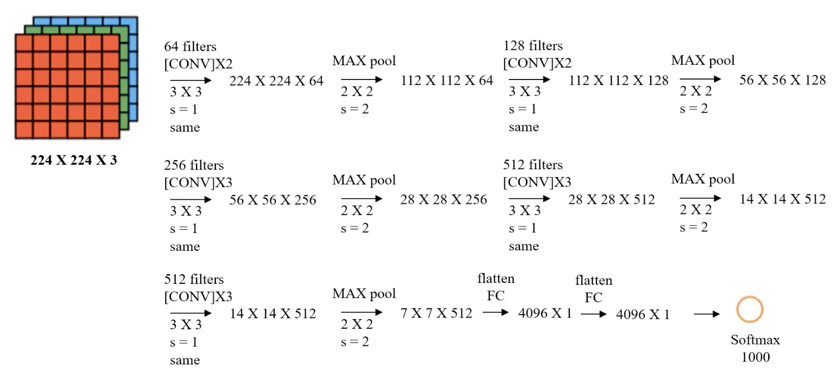
| 层次 | 说明 | 输入尺寸 | 输出尺寸 | 过滤器 | 步长 | 填充 | 激活 |
|---|---|---|---|---|---|---|---|
| 输入层 | RGB 图像 | $224 \times 224 \times 3$ | $224 \times 224 \times 3$ | - | - | - | - |
| Conv1-1 | $3 \times 3$ 卷积 | $224 \times 224 \times 3$ | $224 \times 224 \times 64$ | 64 | 1 | 1 | ReLU |
| Conv1-2 | $3 \times 3$ 卷积 | $224 \times 224 \times 64$ | $224 \times 224 \times 64$ | 64 | 1 | 1 | ReLU |
| Pool1 | 最大池化 | $224 \times 224 \times 64$ | $112 \times 112 \times 64$ | $2 \times 2$ | 2 | 0 | - |
| Conv2-1 | $3 \times 3$ 卷积 | $112 \times 112 \times 64$ | $112 \times 112 \times 128$ | 128 | 1 | 1 | ReLU |
| Conv2-2 | $3 \times 3$ 卷积 | $112 \times 112 \times 128$ | $112 \times 112 \times 128$ | 128 | 1 | 1 | ReLU |
| Pool2 | 最大池化 | $112 \times 112 \times 128$ | $56 \times 56 \times 128$ | $2 \times 2$ | 2 | 0 | - |
(后续层类同)
特征提取后,我们会自己构建MLP模型,有一层隐藏层,10个神经元。
2.4.2. 准备工作
请在终端输入指令以下载和安装:
pip install keras tensorflow scikit-learn
我们的任务是对猫狗进行二分类,会使用到猫狗的照片,这里我们使用Kaggle数据集,各位可以到 kaggle数据集、mnist数据集、imdb数据集分享 这个帖子中找到下载链接,下载好后要先解压。在train文件夹中,创建cat和dog两个文件夹,把猫的照片放到cat中,把狗的照片放到dog中,最后的路径应该长这样:
.\train
	\train
		\dog
			\dog.0.jpg
			\dog.1.jpg
			\dog.2.jpg
			...
		\cat
			\cat.0.jpg
			\cat.1.jpg
			\cat.2.jpg
			...
把train文件夹直接拖入Python项目文件夹中即可。
如果你要在本地实操这个项目,强烈建议在Linux环境下使用带有CUDA加速单元的英伟达GPU,或是AMD GPU手动开启ROCm(仅限Linux)。你当然可以在Windows环境下运行,但是现在的tensorflow不支持Windows平台的GPU加速,所以只能靠纯CPU运算,计算速度会慢很多。我用i9-13900kf要10+分钟,用M1 Max要30分钟。
AMD GPU开启ROCm需要安装适配ROCm的TensorFlow版本(仅支持Linux),可以通过pip直接安装:
pip install tensorflow-rocm
运行以下代码检查TensorFlow是否能检测到AMD GPU:
import tensorflow as tf
print("Num GPUs Available:", len(tf.config.list_physical_devices('GPU')))
2.4.3. 节省内存版代码
Step 1: 初始化VGG-16
# 初始化 VGG 模型(去掉全连接层 MLP)
from tensorflow.keras.applications.vgg16 import VGG16
model = VGG16(weights='imagenet', include_top=False)
weights='imagenet'表示加载的是基于 ImageNet 数据集预训练的权重include_top=False:- 表示不加载 VGG-16 的顶层全连接层(即分类部分),只保留卷积部分
- 这样处理的目的是将 VGG-16 作为一个特征提取器,提取高层次的卷积特征
Step 2: 加载图片
# 定义函数:加载与预处理单张图片
from tensorflow.keras.applications.vgg16 import preprocess_input
import numpy as np
from tensorflow.keras.preprocessing.image import img_to_array, load_img
def load_image_and_preprocess(image_path, model):
    """
    加载图片并进行预处理以适配 VGG 模型
    :param image_path: 图片路径
    :param model: VGG 模型实例
    :return: 预处理后的特征向量
    """
    img = load_img(image_path, target_size=(224, 224))  # 调整图片大小
    img = img_to_array(img)  # 转换为数组
    x = np.expand_dims(img, axis=0)  # 扩展维度以匹配模型输入格式
    x = preprocess_input(x)  # 应用预处理(均值中心化等处理)
    x_vgg = model.predict(x)  # 提取特征
    return np.reshape(x_vgg, (7 * 7 * 512))  # 展平特征

# 定义函数:处理单个文件夹的所有图片
import os
def process_folder(folder, model):
    """
    处理指定文件夹下的所有图片,提取特征向量
    :param folder: 图片文件夹路径
    :param model: VGG 模型实例
    :return: 提取的特征向量数组
    """
    # 获取所有 .jpg 文件路径
    img_paths = [
        os.path.join(folder, file)
        for file in os.listdir(folder)
        if file.endswith('.jpg')
    ]

    # 初始化特征数组(提取完特征之后的形状为 7*7*512)
    features = np.zeros((len(img_paths), 7 * 7 * 512))

    # 遍历所有文件路径,依次加载并提取特征
    for idx, path in enumerate(img_paths):
        features[idx] = load_image_and_preprocess(path, model)
        print(f"Preprocessed: {path}")

    return features, len(img_paths)

# 处理猫图片文件夹
cat_folder = "train/train/cat"
cat_features, cat_count = process_folder(cat_folder, model)  # 猫的特征和数量

# 处理狗图片文件夹
dog_folder = "train/train/dog"
dog_features, dog_count = process_folder(dog_folder, model)  # 狗的特征和数量
定义单张图片的加载与预处理函数 (load_image_and_preprocess):
- 加载指定路径的图片,调整为 VGG16 需要的输入尺寸 224x224。
- 将图片从 PIL 格式转换为 NumPy 数组,并扩展维度以匹配模型的输入格式(4D 张量)。
- 使用
preprocess_input对图片数据进行标准化(VGG16 需要特定格式的输入,如中心化操作)。 - 调用
model.predict使用 VGG16 模型提取特征,得到卷积层输出的特征图,大小为 (7, 7, 512)。 - 展平特征图为一维向量(7×7×512),为后续处理做准备。
定义文件夹中所有图片的处理函数 (process_folder):
- 遍历指定文件夹,筛选出所有以
.jpg结尾的图片文件路径。 - 初始化一个空的特征矩阵 (
features),其大小为 (图片数量, 7×7×512)。 - 对每张图片调用
load_image_and_preprocess,依次提取特征并存储到特征矩阵中。 - 返回提取的特征矩阵以及图片数量。
提取猫和狗图片的特征:
- 指定猫和狗图片存储的文件夹路径(
cat_folder和dog_folder)。 - 分别调用
process_folder对这两个文件夹进行处理,提取每张图片的特征向量,返回特征矩阵(cat_features和dog_features)以及对应的图片数量(cat_count和dog_count)。
Step 3: 生成对应标签
我们需要为训练数据和测试数据提供对应的标签:
# 生成对应的标签(猫为 0,狗为 1)
cat_labels = np.zeros((cat_count, 1))
dog_labels = np.ones((dog_count, 1))

# 合并猫和狗的特征与标签
X = np.concatenate((cat_features, dog_features), axis=0)
y = np.concatenate((cat_labels, dog_labels), axis=0)

# 打印结果信息
print(f"Feature shape: {X.shape}, Label shape: {y.shape}")
输出:
Feature shape: (25000, 25088), Label shape: (25000, 1)
Step 4: 数据分离
我们需要把数据分为训练集和测试集,训练集用于训练模型,测试集用于测试模型的准确率:
# 数据分离
from sklearn.model_selection import train_test_split

X_train, X_test, y_train, y_test = train_test_split(X,
                                                    y,
                                                    test_size=0.2,
                                                    random_state=50)
X: 输入特征矩阵。这里的X是通过 VGG-16 提取并展平后的图片特征,形状为(None, 7 * 7 * 512),用作训练和测试的特征集y: 标签值,即图片所属的类别。这里沿用前文生成的标签,猫为 0,狗为 1test_size=0.2: 表示测试集占整个数据集的比例。在此设置为 20%(即80%用作训练集,20%用作测试集)random_state=50: 随机种子,用于确保数据分割的随机性一致。相同的随机种子保证每次运行程序时,分割出的训练集和测试集相同
Step 5: 建立MLP模型
接下来我们建立自己的MLP模型,有一层隐藏层,10个神经元,输出层有1个神经元表示二分类:
# MLP模型
from keras.models import Sequential
from keras.layers import Dense
model = Sequential()
model.add(Dense(units=10, activation='relu', input_dim=7 * 7 * 512))
model.add(Dense(units=1, activation='sigmoid'))
Step 6: 配置模型
# 配置模型
model.compile(optimizer='adam', loss='binary_crossentropy', metrics=['accuracy'])
-
compile是 Keras 模型的方法,用于在训练模型之前配置模型的学习过程,它的主要参数有:- 损失函数(
loss):定义模型训练时计算误差的方法。 - 优化器(
optimizer):决定模型的参数(如权重和偏置)如何更新,以最小化损失函数。 - 评估指标(
metrics):决定用于评估模型性能的指标,这些指标不会影响模型训练,只用于衡量效果。
- 损失函数(
-
loss='binary_crossentropy':binary_crossentropy(二元交叉熵)是二分类任务中常用的损失函数 -
optimizer='adam':adam(Adaptive Moment Estimation)是一种自适应学习率优化算法,是深度学习中最常用的优化器之一 -
metrics=['accuracy']:指定模型在训练和评估时用准确率来衡量性能
Step 7: 训练模型
把训练集数据喂给模型即可:
# 训练模型
model.fit(X_train, y_train, epochs=50)
Step 8: 评估模型
我们要分别测试训练集和测试集准确率:
# 训练集准确率
train_accuracy = model.evaluate(X_train, y_train)[1]
print('Train Accuracy: ', train_accuracy)

# 测试集准确率
test_accuracy = model.evaluate(X_test, y_test)[1]
print('Test Accuracy: ', test_accuracy)
输出:
Train Accuracy:  0.9991000294685364
Test Accuracy:  0.9833999872207642
效果非常好!
2.4.4. 效率更高版代码
上文中我们将照片一个个处理,这样写的好处在于不占内存,但是效率较低。我们也可以一次性把所有照片加载进内存里一次性处理完,这样写效率更高。
实测,如果采用一次性把所有照片加载进内存的办法将会占用20GB内存,加上IDE(我用的是PyCharm Professional)一共要占23GB内存,也就是说32GB内存才能勉强跑,48GB才能保证不会爆内存。
如果你的电脑内存够大,你可以尝试以下这段代码:
import os
import numpy as np
from tensorflow.keras.preprocessing.image import load_img, img_to_array
from tensorflow.keras.applications.vgg16 import VGG16, preprocess_input

# 初始化 VGG 模型
model = VGG16(weights='imagenet', include_top=False)


def load_and_preprocess_images(folder):
    """
    批量加载并预处理指定文件夹中的所有图片
    :param folder: 图片文件夹路径
    :return: 预处理后的图像批量数据和图像数量
    """
    # 检查路径是否存在
    if not os.path.exists(folder):
        raise FileNotFoundError(f"文件夹不存在:{folder}")

    # 获取所有 .jpg 文件路径
    img_paths = [
        os.path.join(folder, file)
        for file in os.listdir(folder)
        if file.endswith('.jpg')
    ]

    if not img_paths:
        raise ValueError(f"文件夹中未找到图片文件:{folder}")

    # 批量加载所有图片并调整大小为 (224, 224)
    images = np.array([
        img_to_array(load_img(img_path, target_size=(224, 224)))
        for img_path in img_paths
    ])

    # 应用预处理(如均值中心化)
    images = preprocess_input(images)

    print(f"Loaded {len(images)} images from {folder}")
    return images, len(img_paths)


def process_folder_in_batch(folder, model):
    """
    批量处理指定文件夹中的所有图片,提取特征向量
    :param folder: 图片文件夹路径
    :param model: VGG 模型实例
    :return: 提取的特征向量数组和图片数量
    """
    # 加载并预处理所有图片
    images, img_count = load_and_preprocess_images(folder)

    # 批量提取特征向量
    features = model.predict(images)
    features = features.reshape(img_count, -1)  # 展平成 (N, 7*7*512) 的特征矩阵

    print(f"Extracted features for {img_count} images from {folder}")
    return features, img_count

# 路径
BASE_DIR = os.path.abspath("train/train")
cat_folder = os.path.join(BASE_DIR, "cat")
dog_folder = os.path.join(BASE_DIR, "dog")

# 处理猫图片文件夹
try:
    cat_features, cat_count = process_folder_in_batch(cat_folder, model)
except Exception as e:
    print(f"处理猫图片文件夹时发生错误: {e}")

# 处理狗图片文件夹
try:
    dog_features, dog_count = process_folder_in_batch(dog_folder, model)
except Exception as e:
    print(f"处理狗图片文件夹时发生错误: {e}")

# 检查是否成功提取特征
if 'cat_features' in locals() and 'dog_features' in locals():
    # 生成对应的标签(猫为 0,狗为 1)
    cat_labels = np.zeros((cat_count, 1))
    dog_labels = np.ones((dog_count, 1))

    # 合并特征和标签
    X = np.concatenate((cat_features, dog_features), axis=0)
    y = np.concatenate((cat_labels, dog_labels), axis=0)

    print(f"Feature shape: {X.shape}, Label shape: {y.shape}")

    # 数据分离
    from sklearn.model_selection import train_test_split

    X_train, X_test, y_train, y_test = train_test_split(X, y, test_size=0.2, random_state=50)
else:
    print("特征提取失败,无法继续后续处理。")

# 建立MLP模型
from tensorflow.keras.models import Sequential
from tensorflow.keras.layers import Dense
model = Sequential()
model.add(Dense(units=10, activation='relu', input_dim = 7 * 7 * 512))
model.add(Dense(units=1, activation='sigmoid'))

# 配置模型
model.compile(optimizer='adam', loss='binary_crossentropy', metrics=['accuracy'])

# 训练模型
model.fit(X_train, y_train, epochs=50)

# 训练集准确率
train_accuracy = model.evaluate(X_train, y_train)[1]
print('Train Accuracy: ', train_accuracy)

# 测试集准确率
test_accuracy = model.evaluate(X_test, y_test)[1]
print('Test Accuracy: ', test_accuracy)