1.1. Introduction to Multi-Layer Perceptron (Artificial Neural Network)
1.1.1. Why Do We Need a Multi-Layer Perceptron
We have already studied many machine learning algorithms, so why do we still need to learn the multi-layer perceptron?
Let’s look at an example:
Based on the detected data $x_1$, $x_2$ and their labels, determine the category when $x_1 = 0.7$ and $x_2 = 0.6$
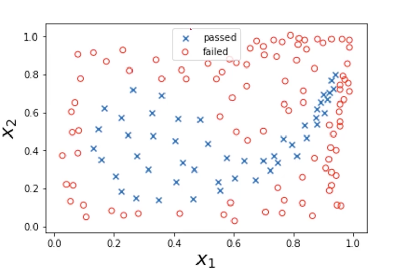
In general, we can build a logistic regression model to find the decision boundary. But here the boundary is obviously very complex, and using logistic regression would require generating a polynomial with a huge number of exponential and term combinations.
In the real world, actual data can only be even more complex than this, and there may be more factors as well. If we still use logistic regression at this point, the computation speed will be very slow.
Let’s take another example:
Automatically identify whether the animal in a picture is a cat or a dog
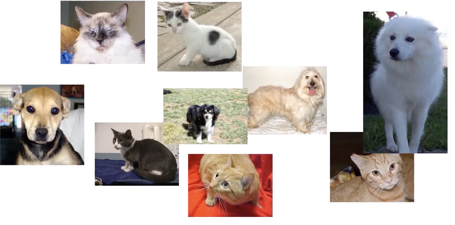
Humans can tell very intuitively which one is a cat and which one is a dog, but computers cannot. To a computer, a photo is just a pile of pixels.
Let’s simplify the task first. Suppose I take two fixed points, $P_1$ and $P_2$, on each image, obtain the grayscale values at these two points, and then plot the data on a Cartesian coordinate system:
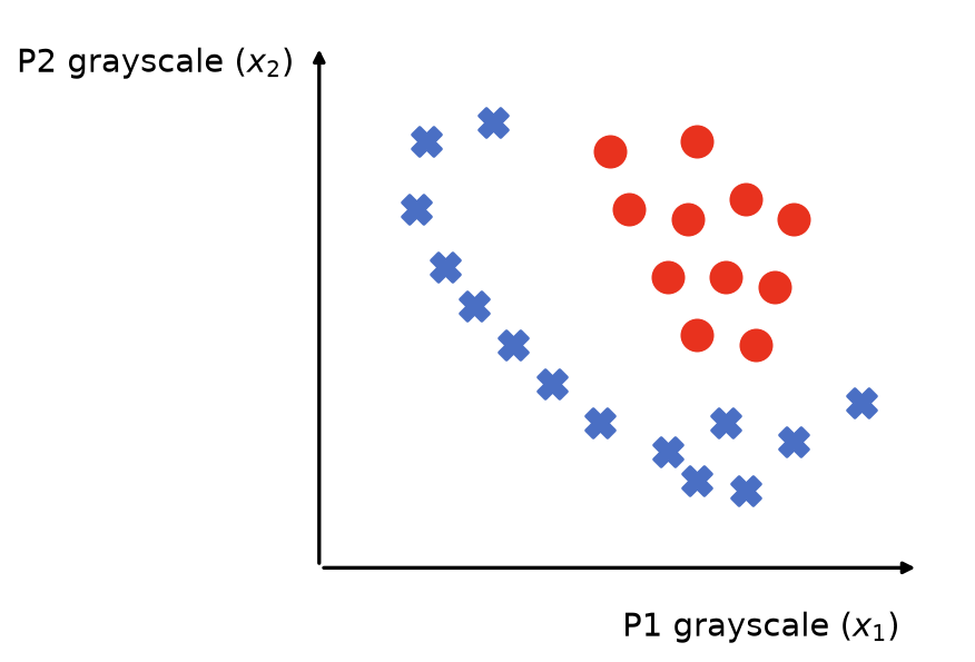
Suppose the red dots represent cats and the blue crosses represent dogs. Then we can let the computer use logistic regression to find the decision boundary that separates cats from dogs. Since we have simplified the task here, the decision boundary does not look very complicated, and logistic regression can handle it.
But in real tasks, we give the computer all pixel grayscale values from a photo. Suppose there is a photo of size 400 x 500, then there will be 200,000 scatter points. At this point, if we use logistic regression, the number of quadratic terms in the model ($x_i \times x_j$) will reach about 20 billion ($\frac{200000 \times 199999}{2}$).
Problems that traditional machine learning cannot handle well are exactly what MLP is used for.
1.1.2. The Core Idea of a Multi-Layer Perceptron (Artificial Neural Network)
The core idea of a multi-layer perceptron (artificial neural network) is to think like a human. So how do humans think?
This involves a bit of biology:
The most basic structural and functional unit in the nervous system is the neuron.
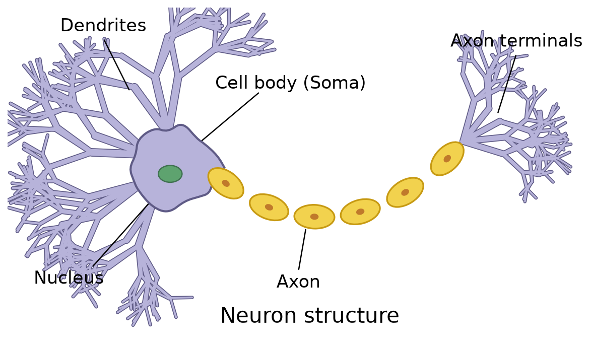
The two most important parts are the dendrites and the axon terminals:
- Dendrites: receive neurotransmitters released by the axon of the previous neuron, causing the neuron to generate a potential difference and transmit information as an electric current
- Axons: release neurotransmitters to the next neuron to pass along information
A multi-layer perceptron (artificial neural network) mimics this basic structure:
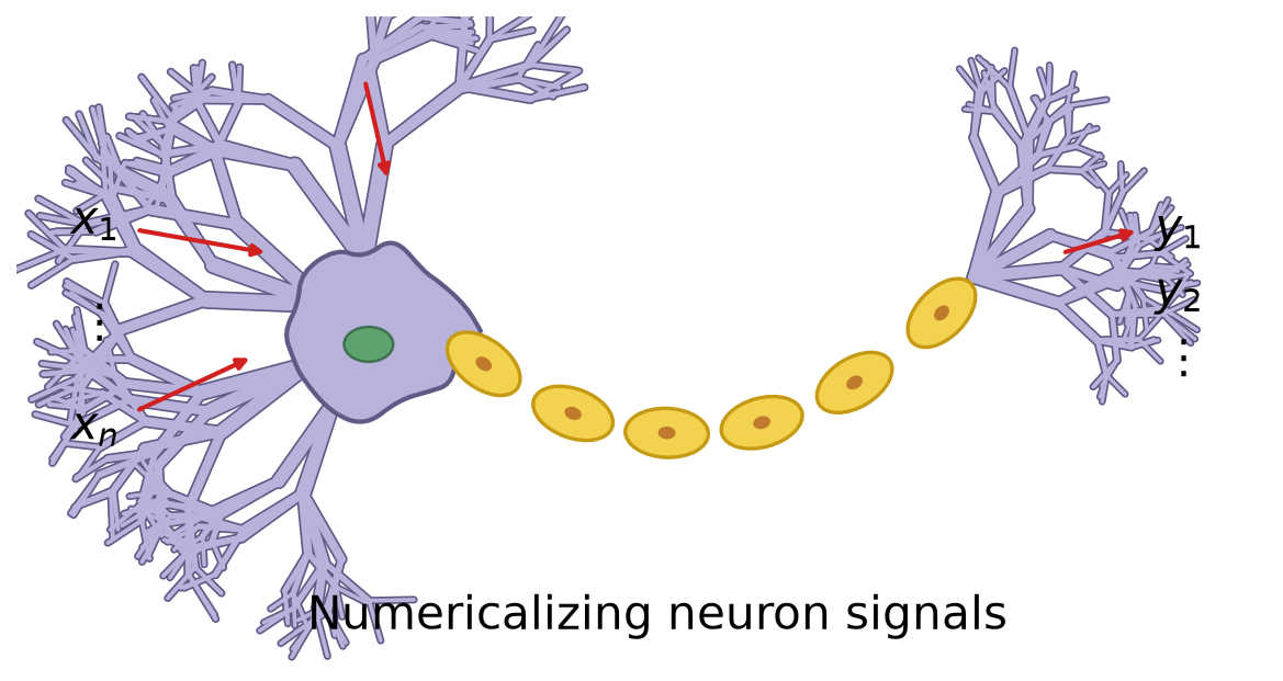
The data are fed into this “neuron” and processed by some formula, producing new data as output.
In fact, this process is very similar to the architecture of logistic regression:
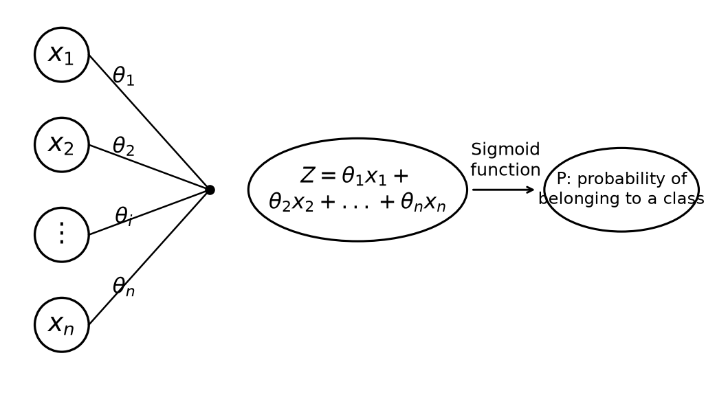
Input data are processed through a formula to produce $P$, and different values of $P$ correspond to different situations.
The human brain is made up of many neurons that form a neural network, and a multi-layer perceptron also relies on many stacked “logistic regression structures” to form an artificial neural network.
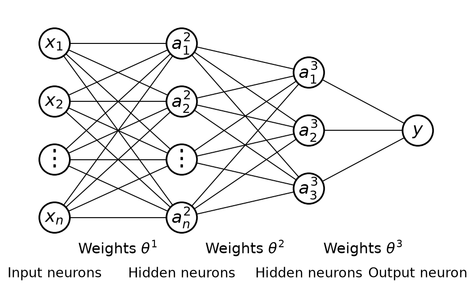
1.1.3. Mathematical Expression of MLP
Input neurons are the input data, and the value of an output neuron determines the probability of belonging to a certain class. Once we know that each neuron node is a logistic regression model, we can derive the hidden neurons between the input neurons and output neurons. Here we take $a_2^2$ as an example: $$ a_2^2 = g\left(\theta_{20}^{1} x_0 + \theta_{21}^{1} x_1 + \theta_{22}^{1} x_2 + \theta_{23}^{1} x_3 \right) $$
- $a_2^2$: represents the activation value of the second neuron in the second layer (the hidden layer), that is, the output
- $g(\cdot)$: represents the activation function, such as sigmoid, ReLU, or tanh. It is used to introduce nonlinearity so that the model can learn complex relationships
- $\theta_{ij}^{1}$: represents the weights between the first layer and the second layer. The superscript 1 here means this is the weight matrix of the first layer (usually the weights from the input layer to the hidden layer). For example, $\theta_{21}^{1}$ represents the weight from the first input node in the input layer to the second neuron in the hidden layer.
- $x_0$, $x_1$, $x_2$, $x_3$: represent the input values, where $x_0$ is usually the bias term, which is generally set to 1.
Some terminology:
- Sigmoid, ReLU, tanh: formulas used to compute nonlinear transformations. Sigmoid is the same formula used in logistic regression, $P(x) = \frac{1}{1 + e^{-x}}$. We will discuss ReLU and tanh later.
- The bias term is like a “freely adjustable number”; it allows a neuron to still produce a nonzero output even when there is no input (or the input is zero), and is used to adjust the neuron’s activation value
As long as we compute each neural node layer by layer in this way, we can obtain the final $y$.
What we need the computer to do is infer the weights from the classified data.
1.2. Multi-Layer Perceptron (Artificial Neural Network) Nonlinear Classification Theory
This article continues from the previous article, 1.1. Introduction to Multi-Layer Perceptron (Artificial Neural Network); please read that one first.
1.2.1. MLP vs. Logistic Regression
What MLP can do, logistic regression can also do. The drawback of logistic regression is that it must add higher-order terms to complete nonlinear classification, which makes it extremely slow. So our goal is to use MLP to perform classification without adding higher-order terms.
1.2.2. An Example
Let’s take an example. Suppose our final goal is to classify these points:
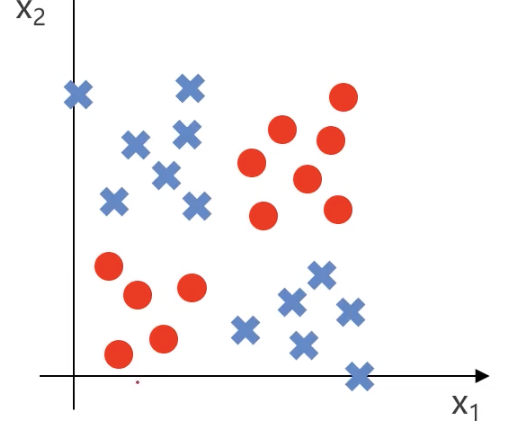
We can simplify the model first: red points appear in the lower left and upper right corners, while blue points appear in the upper left and lower right corners:
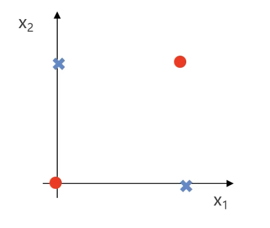
Suppose red points are valued as 1 and blue points as 0. Then we can get the following truth table:
| X₁ | X₂ | y |
|---|---|---|
| 0 | 0 | 1 |
| 0 | 1 | 0 |
| 1 | 0 | 0 |
| 1 | 1 | 1 |
- When $x_1$ and $x_2$ are both 0 or both 1, the result is 1
- When $x_1$ and $x_2$ are different, the result is 0
In professional mathematical terms, $y$ is the XNOR gate of $x_1$ and $x_2$ ($y: x_1 \text{ XNOR } x_2$).
1.2.3. Logic Gates
AND Gate
The XNOR gate mentioned above is one kind of logic gate. Let’s first talk about the most basic logic gate, the AND gate ($AND$): only when $x_1$ and $x_2$ are both true (1) does the result become true (1); in all other cases it is false (0).
Suppose we have the following input factors: $x_0 = 1$, $x_1$, and $x_2$
- $x_0$ is usually the bias term, and is generally set to 1. The bias term is like a “freely adjustable number”; it allows a neuron to still produce a nonzero output even when there is no input (or the input is zero), and is used to adjust the neuron’s activation value
Let the weights of each input be $\theta_{10}^1$, $\theta_{11}^1$, and $\theta_{12}^1$. Multiply each input by its weight, add them up, and then apply the logistic function to obtain the neuron output: $$ y = h(\theta, x) = g\left(\theta_{10}^{1} + \theta_{11}^{1} x_1 + \theta_{12}^{1} x_2\right) $$
- $\theta_{ij}^{1}$: represents the weights between the first layer and the second layer. The superscript 1 here means this is the weight matrix of the first layer (usually the weights from the input layer to the hidden layer). For example, $\theta_{11}^{1}$ represents the weight from the first input node in the input layer to the first neuron in the hidden layer.
Where: $$ g(x) = \frac{1}{1 + e^{-x}} $$
If we set the weights to $\theta_{10}^1 = -20$, $\theta_{11}^1 = 15$, and $\theta_{12}^1 = 15$, this neuron can implement the AND gate. We can first substitute these parameters into the formula: $$ h(\theta, x) = g\left(-20 + 15x_1 + 15x_2\right) $$
Let’s compute the value for each case:
| x₁ | x₂ | $h(\theta, x)$ | y |
|---|---|---|---|
| 0 | 0 | $g(-20)$ | 0 |
| 0 | 1 | $g(-5)$ | 0 |
| 1 | 0 | $g(-5)$ | 0 |
| 1 | 1 | $g(10)$ | 1 |
Only when both $x_1$ and $x_2$ are 1 is the $y$ value 1. This shows that the neuron implements the AND gate.
Neither $x_1$ Nor $x_2$
Next, let’s look at a more complex logic gate: how do we express “neither $x_1$ nor $x_2$”? In this phrase, “neither” means NOT, and “nor” means AND.
So the logic gate expression should be: $y$: $NOT(x_1)$ $AND$ $NOT(x_2)$
By changing the weights, we can modify the neuron above so that it outputs the logic of neither $x_1$ nor $x_2$: $$ h(\theta, x) = g\left(5 - 10x_1 - 10x_2\right) $$
Let’s plug in the data:
| x₁ | x₂ | $h(θ, x)$ | y |
|---|---|---|---|
| 0 | 0 | $g(5)$ | 1 |
| 0 | 1 | $g(-5)$ | 0 |
| 1 | 0 | $g(-5)$ | 0 |
| 1 | 1 | $g(-15)$ | 0 |
OR Gate
If we want to implement an OR gate ($y:$ $x_1$ $OR$ $x_2$): if either $x_1$ or $x_2$ is 1, the final result is 1. We can set the weights like this: $$ h(\theta, x) = g\left(-10 + 15x_1 + 15x_2\right) $$
Let’s plug in the data:
| x₁ | x₂ | $h(θ, x)$ | y |
|---|---|---|---|
| 0 | 0 | $g(-10)$ | 0 |
| 0 | 1 | $g(5)$ | 1 |
| 1 | 0 | $g(5)$ | 1 |
| 1 | 1 | $g(20)$ | 1 |
1.2.4. Logic Gates and MLP
$y:$ $x_1$ $AND$ $x_2$
graph TD;
    A[1] -->| -20 | D[y]
    B[x₁] -->| 15 | D[y]
    C[x₂] -->| 15 | D[y]
$y$: $NOT(x_1)$ $AND$ $NOT(x_2)$
graph TD;
    A[1] -->| 5 | D[y]
    B[x₁] -->| -10 | D[y]
    C[x₂] -->| -10 | D[y]
$y:$ $x_1$ $OR$ $x_2$
graph TD;
    A[1] -->| -10 | D[y]
    B[x₁] -->| 15 | D[y]
    C[x₂] -->| 15 | D[y]
By combining these logic gates in different arrangements, we can build a more complex MLP model and thus realize the original XNOR gate ($y: x_1 \text{ XNOR } x_2$) logic.
How do we do that? The logic is as follows:
graph TD;
    %% Input Layer
    A[1] -->| 5 | B[a₁²]
    A[1] -->| -20 | C[a₂²]
    X1[x₁] -->| -10 | B[a₁²]
    X1[x₁] -->| 15 | C[a₂²]
    X2[x₂] -->| -10 | B[a₁²]
    X2[x₂] -->| 15 | C[a₂²]

    %% Hidden Layer to Output Layer
    B[a₁²] -->| 15 | Y[y]
    C[a₂²] -->| 15 | Y[y]
    Bias2[1] -->| -10 | Y[y]
This may look a little confusing, so let me explain step by step:
- The value of $a_1^2$ is the result of the “neither $x_1$ nor $x_2$” logic for $x_1$ and $x_2$
- The value of $a_2^2$ is the result of the AND gate for $x_1$ and $x_2$
- The value of $y$ is the OR gate result of $a_1^2$ and $a_2^2$
Let’s plug in the data and see whether this setup can achieve the effect of the XNOR gate:
| x₁ | x₂ | a₁² | a₂² | $h(θ, x)$ | y |
|---|---|---|---|---|---|
| 0 | 0 | 1 | 0 | $g(5)$ | 1 |
| 0 | 1 | 0 | 0 | $g(-10)$ | 0 |
| 1 | 0 | 0 | 0 | $g(-10)$ | 0 |
| 1 | 1 | 0 | 1 | $g(5)$ | 1 |
1.2.5. Solving the Problem
What we just solved was the classification problem of the simplified model:
So how does the machine iterate toward something like this XNOR-gate effect? We only need to let the model keep iterating to obtain the classification of the final example:
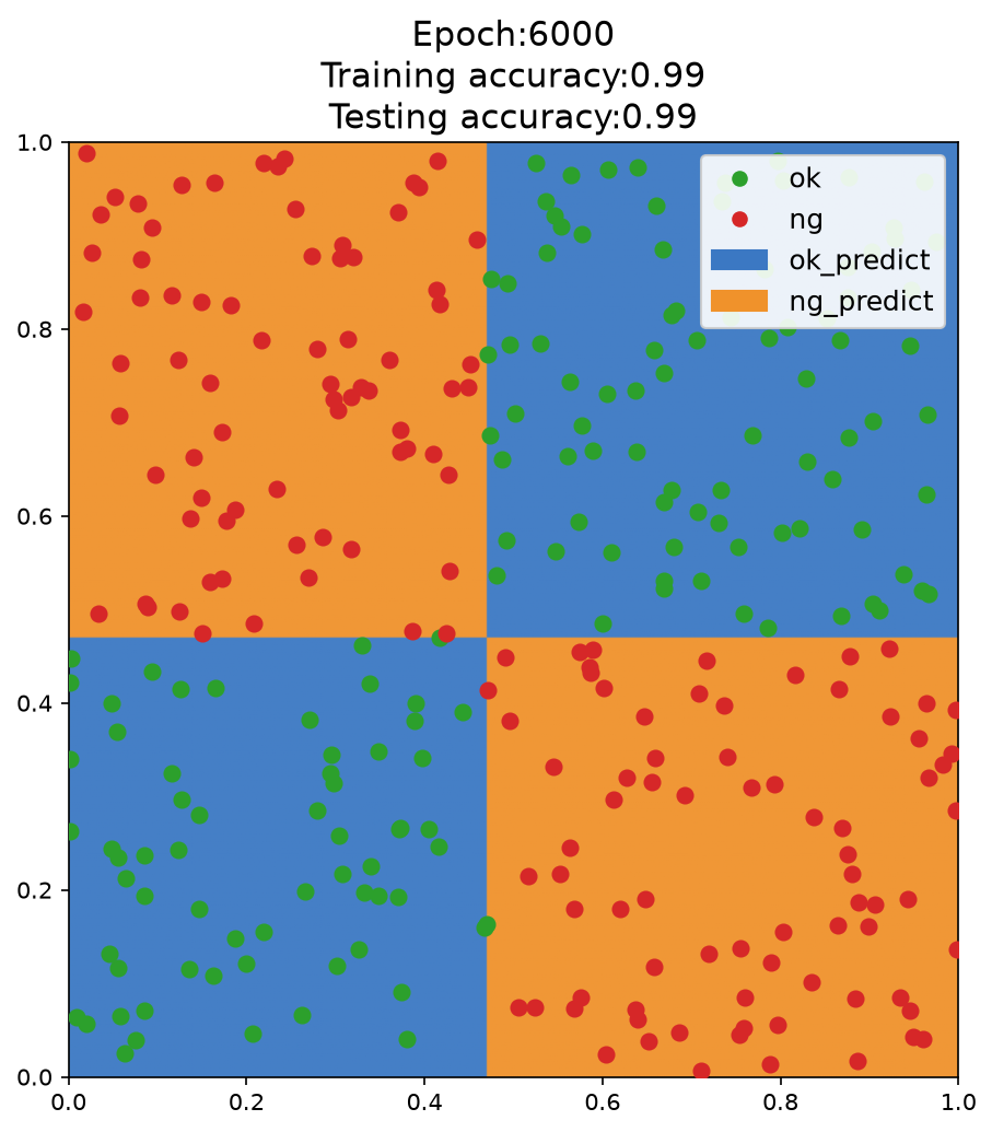
How exactly does the iteration work? (1) Randomly initialize the weights
- The initial weights of the MLP (multi-layer perceptron) are randomly initialized, which means the decision boundary at the beginning is random and may not have any practical meaning.
(2) Forward propagation to compute outputs
- Compute the output after the input $x_1$ and $x_2$ pass through the hidden layer and activation function.
- Compute the final predicted value $y$ of the MLP.
- Compare it with the true label $y_{\text{true}}$ and compute the loss function, such as cross-entropy loss or mean squared error.
(3) Error computation and backpropagation
- Use Backpropagation to calculate each weight’s contribution to the error.
- Use Gradient Descent or Adam to update the parameters so that the model’s predictions become closer to the true labels.
(4) After several rounds of iteration:
- The MLP gradually learns which regions should output 1 and which regions should output 0.
- The hidden layer neurons learn basic features, such as certain regions corresponding to the AND gate and others corresponding to the OR gate, eventually combining into an XNOR model.
- During training, the decision boundary gradually approaches the real classification boundary, eventually forming a nonlinear separating surface similar to the one shown by the boundary between the blue and orange regions in the figure.
1.2.6. MLP for Multi-Classification
In real life, data are not limited to just two cases; there can be many. In that case, we need MLP to perform multi-class classification.
Let’s recall the basic framework of MLP:
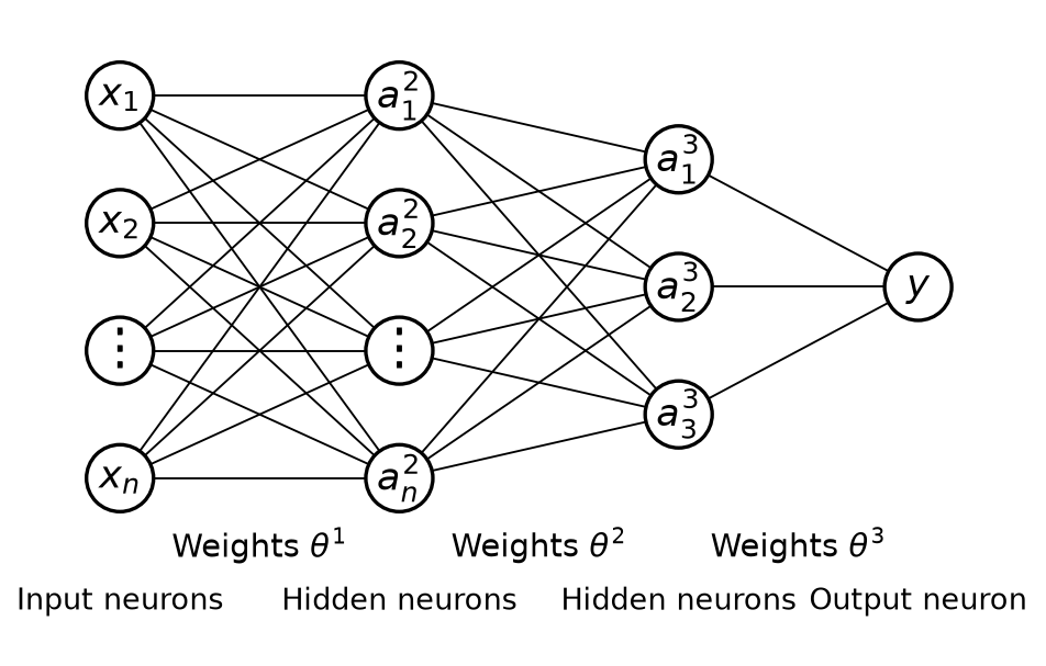
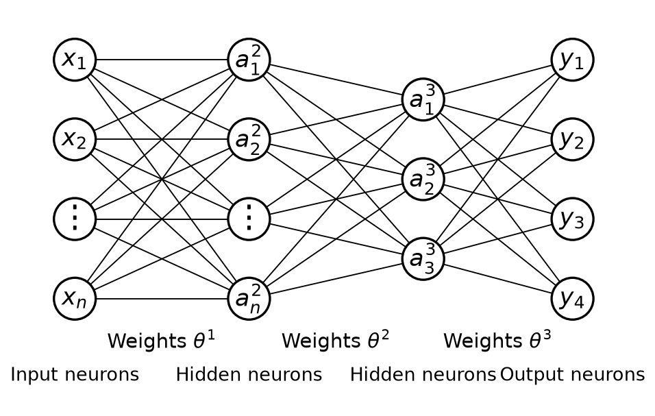
We can implement multi-class classification by outputting several neurons. Suppose there are 4 classes, then we set up 4 output neurons: $y_1$, $y_2$, $y_3$, and $y_4$. After inputting the data, we obtain the outputs of these 4 neurons, which are the probabilities that the data belongs to each class. We simply choose the one with the highest probability as the prediction result, as shown below:
1.3. Using Keras to Implement Multi-Layer Perceptron (Artificial Neural Network) Hands-On (Basics)
This article continues from the previous article, 1.2. Multi-Layer Perceptron (Artificial Neural Network) Nonlinear Classification Theory; please read that one first.
1.3.1. Keras
Keras is an application programming interface written in Python for neural network development. By using this API, you can develop neural networks, convolutional neural networks, recurrent neural networks, and other common deep learning algorithms.
Features:
- It integrates many mature deep learning algorithms, is easy to install and use, comes with abundant examples, and has very detailed tutorials and documentation
- It can run with TensorFlow or Theano as its backend
I have attached the official website here.
1.3.2. Relationship Between Keras and TensorFlow
TensorFlow is an open-source software library that uses a data-flow graph and is used for numerical computation. It can automatically compute derivatives related to a model, which makes it very suitable for solving neural network models.
Keras can be seen as an interface encapsulated on top of TensorFlow (Keras as the front end, TensorFlow as the back end). Keras provides users with an easy-to-interact-with shell that makes rapid deep learning development convenient.
1.3.3. Install Keras and TensorFlow
Enter the following command in the terminal to download and install them:
pip install keras tensorflow
1.3.4. Preparation
This article uses my csv file. I uploaded it to GitHub, and you can click the link to view and download it.
It has 3 columns of information: one column is x1, one column is x2, and these two columns represent the two input variables. The other column is label, and the values in this column are either 0 or 1.
After downloading it, just move it into your Python project folder.
1.3.5. Write the Code
Step 1: Load the Data
First, use the pandas library to read the data:
# Read the data
import pandas as pd
data = pd.read_csv('scatter_data.csv')
Visualize it with matplotlib:
# Visualize the raw data
# Draw the scatter plot
import matplotlib.pyplot as plt

scatter = plt.scatter(
    data['x1'],
    data['x2'],
    c = ['blue' if label == 0 else 'red' for label in data['label']],
)

plt.show()
Image output:
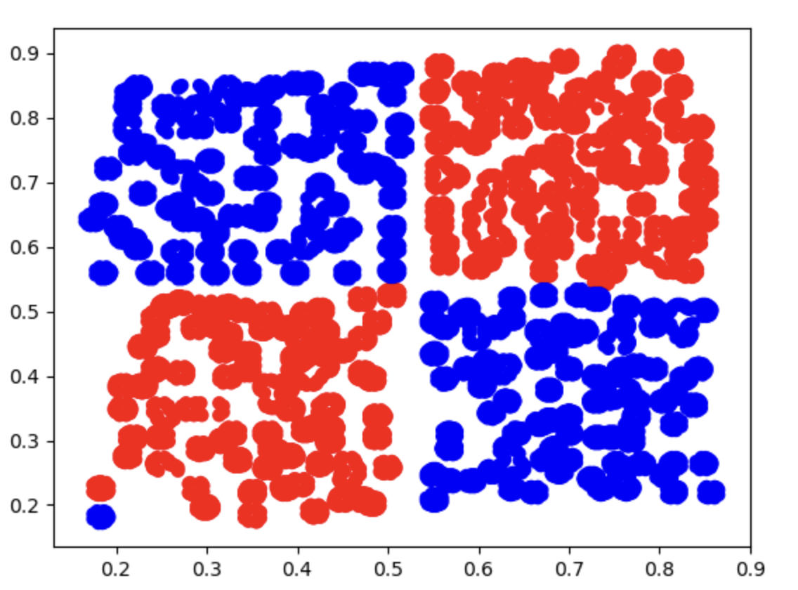
Step 2: Assign Values to x and y
- The value of
xcorresponds to the two input valuesx1andx2 - The value of
ycorresponds to the labellabel
# Assign values to x and y
x = data.drop(['label'], axis=1)
y = data.loc[:,'label']
We also need to split the data into training and test sets for later model evaluation:
# Split into training and test sets
from sklearn.model_selection import train_test_split
x_train, x_test, y_train, y_test = train_test_split(x, y, test_size=0.3, random_state=10)
Step 3: Create the Model
We need to create an MLP with three layers to solve the problem, and each neuron uses the logistic function. Its rough structure should look like this flowchart:
graph TD;
    %% Input Layer
    A[1] -->| 5 | B[a₁²]
    A[1] -->| -20 | C[a₂²]
    X1[x₁] -->| -10 | B[a₁²]
    X1[x₁] -->| 15 | C[a₂²]
    X2[x₂] -->| -10 | B[a₁²]
    X2[x₂] -->| 15 | C[a₂²]

    %% Hidden Layer to Output Layer
    B[a₁²] -->| 15 | Y[y]
    C[a₂²] -->| 15 | Y[y]
    Bias2[1] -->| -10 | Y[y]
# Build a Sequential model
from keras.models import Sequential
model = Sequential()

# Stack layers with add
from keras.layers import Dense
model.add(Dense(units=20, activation='sigmoid', input_dim=2)) # From the first layer (input layer) to the second layer (hidden layer)
model.add(Dense(units=1, activation='sigmoid')) # From the second layer (hidden layer) to the third layer (output layer)

# View the model structure
model.summary()

# Configure model-solving parameters with .compile()
model.compile(loss='binary_crossentropy', optimizer='adam', metrics=['accuracy'])
-
Sequentialis a basic model type in Keras used to stack network layers one after another, with each layer connected in creation order. This approach is ideal for building neural networks that follow a single path from input to output, such as classic feedforward neural networks -
The first
addadds aDenselayer (a hidden layer):- Fully connected layer, where each neuron is connected to every neuron in the previous layer
units=20: indicates that the hidden layer contains 20 neuronsactivation='sigmoid': uses the logistic function as the activation function, which maps input values into the range (0, 1) and is suitable for binary classification or probability outputsinput_dim=2: indicates that the input feature dimension is 2 (x1andx2), which is the input shape of the first layer
-
The second
addadds the output layer:units=1: indicates that this layer has only one neuron, i.e. the output dimension is 1activation='sigmoid': in the output layer, sigmoid is commonly used as the activation function for binary classification problems, producing values between 0 and 1 that represent the probability of belonging to a certain class
-
model.summary(): prints detailed structural information about the neural network model, including each layer’s name, output shape, and parameter count. This is an important method for debugging and understanding the model, and it helps confirm that the model you built matches your intended design -
.compile()defines the training configuration of the model, including the loss function, optimizer, and evaluation metrics:loss='binary_crossentropy': the loss function. Choose the appropriate loss based on the task.binary_crossentropyis generally used for binary classificationoptimizer='adam': the optimizer, here Adam (Adaptive Moment Estimation)metrics=['accuracy']: the evaluation metric; here accuracy is selected as the evaluation criterion
Output:
Model: "sequential"
┏━━━━━━━━━━━━━━━━━━━━━━━━━━━━━━━━━┳━━━━━━━━━━━━━━━━━━━━━━━━┳━━━━━━━━━━━━━━━┓
┃ Layer (type)                    ┃ Output Shape           ┃       Param # ┃
┡━━━━━━━━━━━━━━━━━━━━━━━━━━━━━━━━━╇━━━━━━━━━━━━━━━━━━━━━━━━╇━━━━━━━━━━━━━━━┩
│ dense (Dense)                   │ (None, 20)             │            60 │
├─────────────────────────────────┼────────────────────────┼───────────────┤
│ dense_1 (Dense)                 │ (None, 1)              │            21 │
└─────────────────────────────────┴────────────────────────┴───────────────┘
 Total params: 81 (324.00 B)
 Trainable params: 81 (324.00 B)
 Non-trainable params: 0 (0.00 B)
Step 4: Train the Model
We just need to feed the data into the model and let it iterate:
model.fit(x_train, y_train, epochs=3000)
- The
epochsparameter controls the number of iterations
Step 5: Predict the Data
We use the x values in the test set to predict the y values and compare them with the actual y values to generate accuracy:
# Predicted values
y_predict = model.predict(x_test)

# Convert probability values into discrete class labels
y_predict_classes = (y_predict > 0.5).astype(int)

# Calculate accuracy
from sklearn.metrics import accuracy_score

print(accuracy_score(y_test, y_predict_classes))
Output:
0.9977413890457368
If we keep iterating, the accuracy will be even higher, but it may cause overfitting, which would not be worth it.
1.4. Multi-Layer Perceptron (Artificial Neural Network) Handwritten Digit Recognition (Image Multi-Classification)
This article continues from the previous article, 1.3. Using Keras to Implement Multi-Layer Perceptron (Artificial Neural Network) Hands-On (Basics); please read that one first.
1.4.1. MNIST Dataset
In this article, we will use the MNIST dataset to build an MLP model and recognize handwritten digits from 0 to 9.
The MNIST (Modified National Institute of Standards and Technology) dataset is a handwritten digit recognition dataset used to train and test machine learning models. It consists of 70,000 grayscale images, of which:
- Training Set: 60,000 images
- Test Set: 10,000 images
Each image is a 28×28 grayscale image representing a handwritten digit between 0 and 9. The labels are integers from 0 to 9, indicating the digit category shown in the image.
We use it because:
- Standardized: all images have the same size (28×28 pixels)
- Easy to use: suitable as an introductory dataset for deep learning
- Widely used: used to test the performance of various machine learning and deep learning models, such as CNNs (convolutional neural networks), SVMs (support vector machines), and more
1.4.2. Preparation
This article uses keras, tensorflow, and matplotlib. If you do not have them installed, please install them.
Enter the following command in the terminal to download and install them:
pip install keras tensorflow matplotlib
1.4.3. Write the Code
Step 1: Import the MNIST Dataset
Keras already includes the MNIST dataset, so we can import it directly:
from keras.datasets import mnist
(x_train, y_train),(x_test, y_test) = mnist.load_data()
The first time you use the dataset, the program will download the resources from the official website, so you will need to wait a moment. Let’s take a look at some information about the data:
print(type(x_train), x_train.shape)
<class 'numpy.ndarray'> (60000, 28, 28)
- Its type is a
numpyarray - It contains 60,000 samples, and each sample is 28 by 28 pixels
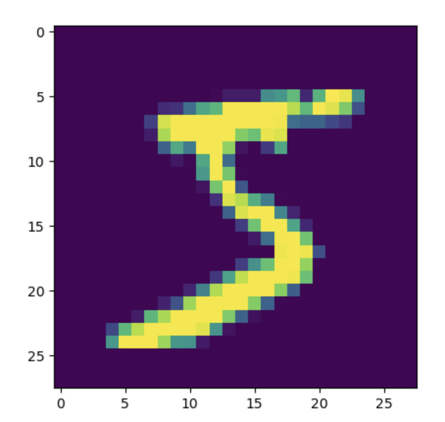
We can use matplotlib to see what the data looks like:
# Visualize the input data
from matplotlib import pyplot as plt
plt.imshow(x_train[0])
plt.show()
Output image:
Step 2: Array Conversion
We need to convert each image from a 28-by-28 two-dimensional array into a one-dimensional array with 784 elements so that the MLP can receive it:
# Convert the data
feature_size = x_train.shape[1] * x_train.shape[2]
x_train = x_train.reshape(x_train.shape[0], feature_size)
x_test = x_test.reshape(x_test.shape[0], feature_size)
- The original shape is
(number of samples, height, width), which represents the data for each image. After conversion, the shape becomes(number of samples, feature size), flattening all pixels into a one-dimensional feature vector so that each image can be processed as a sample by the model feature_sizecorresponds to the feature size, that is, the number of pixels in a single image. You can get it withx_train.shape[1] * x_train.shape[2]reshapeis a method in NumPy used to adjust the shape of an array. It is often used to reshape matrices or tensors without changing the data itself. This method does not modify the original array; instead, it returns a new array that shares memory with the original data
We can print the structure of the data at this point:
print(x_train.shape)
Output:
(60000, 784)
Step 3: Data Normalization
The images in the MNIST dataset are 8-bit grayscale images, and the pixel values range from 0 to 255. Nonlinear activation functions used in MLP models, such as sigmoid, tanh, and ReLU, are sensitive to value ranges. So we need to normalize the data and shrink the range.
In general, dividing the grayscale pixel values by 255 is enough. This keeps the values between 0 and 1, which is more suitable for an MLP model:
# Normalize the data
x_train = x_train.astype('float32')
x_test = x_test.astype('float32')
x_train /= 255
x_test /= 255
astype('float32'): after loading, the pixel values in the MNIST dataset are integers (0to255).astype('float32')converts them to floating-point values so that more precise mathematical operations, such as normalization and gradient updates, can be performedx_train /= 255andx_test /= 255: divide the pixel values by 255 so that the range is compressed from[0, 255]to[0, 1]
Step 4: Convert the Label Format
The model output labels will use one-hot encoding: each class is assigned one position, with the specific class position set to 1 and all others set to 0. Suppose there are 3 classes: A, B, and C, then:
- Class
Ais encoded as[1, 0, 0] - Class
Bis encoded as[0, 1, 0] - Class
Cis encoded as[0, 0, 1]
The original label format is integer labels: for example, if the image is a handwritten 5, the corresponding label value is 5.
Because these two storage formats are different, it becomes troublesome to compare labels and evaluate the model. We need to convert the original integer labels into one-hot encoding.
Suppose our label is 5. We need to store “5” like this:
[0, 0, 0, 0, 0, 1, 0, 0, 0, 0]
To represent 5, write 1 in the 6th position (the first position is 0, so the placement of each digit must be shifted by 1), and set the rest to 0.
keras provides the to_categorical function for converting label formats:
# Convert the label format
from keras.utils import to_categorical
y_train = to_categorical(y_train)
y_test = to_categorical(y_test)
Step 5: Build the Model
After completing all the data preprocessing work mentioned above, we can build the model! Our input has 784 features (corresponding to the number of pixels), the second layer will be reduced by half to 392 neurons, the third layer will still keep 392 neurons, and the fourth layer, which is the output layer, needs 10 output neurons corresponding to 0 through 9:
# Build the model
from keras.models import Sequential
from keras.layers import Dense

model = Sequential()
model.add(Dense(units=392, activation='sigmoid', input_dim=feature_size))
model.add(Dense(units=392, activation='sigmoid'))
model.add(Dense(units=10, activation='softmax'))
-
units=392: indicates that this layer has 392 neurons (hidden nodes) -
input_dim=feature_size: the input dimension, which indicates how many features the layer receives. This corresponds to the previous input-layer shape(number of samples, feature_size), wherefeature_size = 784(after each MNIST image is converted into a feature vector, it has 784 pixels). Starting from the second layer, there is no need to explicitly declareinput_dim, because the input shape is automatically inferred from the output of the previous layer (the first hidden layer) -
Softmax activation function maps the values of the output neurons (logits) into a probability distribution, making it suitable for multi-class classification problems
Let’s use the summary method to display the structure:
model.summary()
Output:
Model: "sequential"
┏━━━━━━━━━━━━━━━━━━━━━━━━━━━━━━━━━┳━━━━━━━━━━━━━━━━━━━━━━━━┳━━━━━━━━━━━━━━━┓
┃ Layer (type)                    ┃ Output Shape           ┃       Param # ┃
┡━━━━━━━━━━━━━━━━━━━━━━━━━━━━━━━━━╇━━━━━━━━━━━━━━━━━━━━━━━━╇━━━━━━━━━━━━━━━┩
│ dense (Dense)                   │ (None, 392)            │       307,720 │
├─────────────────────────────────┼────────────────────────┼───────────────┤
│ dense_1 (Dense)                 │ (None, 392)            │       154,056 │
├─────────────────────────────────┼────────────────────────┼───────────────┤
│ dense_2 (Dense)                 │ (None, 10)             │         3,930 │
└─────────────────────────────────┴────────────────────────┴───────────────┘
 Total params: 465,706 (1.78 MB)
 Trainable params: 465,706 (1.78 MB)
 Non-trainable params: 0 (0.00 B)
Step 6: Configure the Model
When configuring the model, we can choose whether it is a binary classification or multi-class classification model, and which optimization algorithm to use:
# Configure the model
model.compile(loss='categorical_crossentropy', optimizer='adam', metrics=['accuracy'])
-
compileis a Keras model method used to configure the learning process before training. Its main parameters are:- Loss function (
loss): defines how errors are computed during training. - Optimizer (
optimizer): determines how the model’s parameters, such as weights and biases, are updated to minimize the loss function. - Evaluation metrics (
metrics): determine the metrics used to evaluate model performance. These metrics do not affect training; they are only used to measure results.
- Loss function (
-
loss='categorical_crossentropy':categorical_crossentropy(categorical cross-entropy) is a commonly used loss function for multi-class tasks -
optimizer='adam':adam(Adaptive Moment Estimation) is an adaptive learning-rate optimization algorithm and one of the most commonly used optimizers in deep learning -
metrics=['accuracy']: specifies accuracy as the metric used to measure performance during training and evaluation
Step 7: Train the Model
We just need to feed the training data into the model:
# Train the model
model.fit(x_train, y_train, epochs=10)
- The
epochsparameter controls the number of iterations
Compared with the previous article, this time we chose a much smaller number of iterations (the previous one was 3,000 iterations, while this one only has 10). This is because our image data are very large (60,000 samples), so we can get good results without many iterations. However, each iteration will take longer.
Step 8: Evaluate the Model
We use accuracy to evaluate the model.
Since Step 4 already converted the labels to one-hot encoding, we can evaluate by using argmax to recover class indices from both the predicted probabilities and the true labels, then comparing them:
# Training set accuracy
import numpy as np
y_train_predict = model.predict(x_train)
y_train_pred_classes = np.argmax(y_train_predict, axis=1)
y_train_true_classes = np.argmax(y_train, axis=1)
train_accuracy = np.mean(y_train_pred_classes == y_train_true_classes)
print("Training set accuracy:", train_accuracy)

# Test set accuracy
y_test_predict = model.predict(x_test)
y_test_pred_classes = np.argmax(y_test_predict, axis=1)
y_test_true_classes = np.argmax(y_test, axis=1)
test_accuracy = np.mean(y_test_pred_classes == y_test_true_classes)
print("Test set accuracy:", test_accuracy)
np.argmax(..., axis=1): for each row, take the class index with the highest probability. For example, a prediction[0.1, 0.8, 0.1, ...]becomes class1- Compare predicted classes with true classes sample by sample, then use
np.meanto get the proportion that match, which is the accuracy
Output:
Training set accuracy: 0.9979166666666667
Test set accuracy: 0.9808
2.1. Convolutional Neural Network (CNN) Model Theory (Basic) - Convolution, Pooling, and ReLU Function
2.1.1. Computational Cost Problem
The original motivation for introducing MLPs was to solve the problem of excessive computation in logistic regression.
Take handwritten digit recognition as an example. For a 28×28 image:
- A logistic regression model with a cubic polynomial decision boundary has 80,931,145 trainable parameters
- An MLP model with 784 input features, two hidden layers with 394 hidden neurons each, and 10 output neurons has 465,706 trainable parameters
But this is only a very small grayscale image. If we use an RGB image with both width and height above 100 pixels in daily life, such as 500×400, for binary classification, we would need 78,558,378 trainable parameters. That is still far too much computation.
So is there a more computationally efficient way? That is where convolutional neural networks come in.
2.1.2. Image Convolution
Think about what a computer mainly looks at when performing object recognition: contours, right? MLPs are computationally expensive because there are too many contours in the image for the computer to process. If we can first extract the main contours in the image, that is, the most critical information, and then let the MLP analyze them, we can greatly reduce the computational burden.
The step of extracting the main information requires image convolution. Image convolution refers to multiplying corresponding elements of an image matrix and a filter matrix, then summing the result to form a new matrix. Its main purpose is to quickly locate certain edge features in an image.
Mathematically, the convolution of A and B is usually written as: $$ A \ast B $$ or: $$ convolution(A, B) $$
Let us look at an example:
We have a 7×7 two-dimensional array representing an image: $$ A =
\begin{bmatrix}
X_{11} & X_{12} & X_{13} & X_{14} & X_{15} & X_{16} & X_{17} \
X_{21} & X_{22} & X_{23} & X_{24} & X_{25} & X_{26} & X_{27} \
X_{31} & X_{32} & X_{33} & X_{34} & X_{35} & X_{36} & X_{37} \
X_{41} & X_{42} & X_{43} & X_{44} & X_{45} & X_{46} & X_{47} \
X_{51} & X_{52} & X_{53} & X_{54} & X_{55} & X_{56} & X_{57} \
X_{61} & X_{62} & X_{63} & X_{64} & X_{65} & X_{66} & X_{67} \
X_{71} & X_{72} & X_{73} & X_{74} & X_{75} & X_{76} & X_{77}
\end{bmatrix} $$
We also have a 3×3 filter: $$ F =
\begin{bmatrix}
W_{11} & W_{12} & W_{13} \
W_{21} & W_{22} & W_{23} \
W_{31} & W_{32} & W_{33}
\end{bmatrix} $$ Performing the $A \ast B$ operation looks like this (this figure uses image padding, but here we will treat it as the original 7×7 size; we will talk about padding in the next article (2.2. Convolutional Neural Network (CNN) Model Theory (Advanced) - Image Padding, LeNet, and AlexNet)):
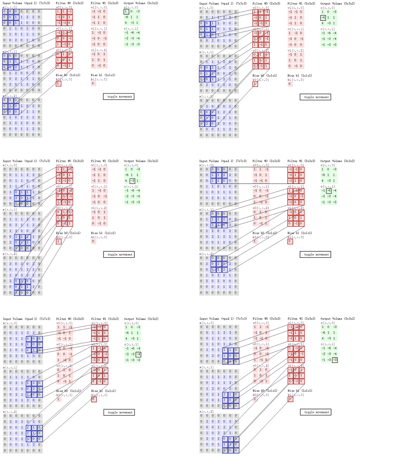
The filter is like a mask covering the image. Wherever it covers, convolution is performed there, moving pixel by pixel.
Suppose the filter is now in the upper-left corner of the image and covers: $$ \begin{bmatrix}
X_{11} & X_{12} & X_{13} \ X_{21} & X_{22} & X_{23} \ X_{31} & X_{32} & X_{33} \
\end{bmatrix} $$ Then the convolution operation performed there, multiplying and summing, is: $$ Y_{11} = X_{11} W_{11} + X_{12} W_{12} + X_{13} W_{13} + X_{21} W_{21} + X_{22} W_{22} + X_{23} W_{23} + X_{31} W_{31} + X_{32} W_{32} + X_{33} W_{33} $$
If we convolve the entire matrix, we will get a smaller matrix, from 7×7 down to 5×5: $$ Y = \begin{bmatrix} Y_{11} & Y_{12} & Y_{13} & Y_{14} & Y_{15} \ Y_{21} & Y_{22} & Y_{23} & Y_{24} & Y_{25} \ Y_{31} & Y_{32} & Y_{33} & Y_{34} & Y_{35} \ Y_{41} & Y_{42} & Y_{43} & Y_{44} & Y_{45} \ Y_{51} & Y_{52} & Y_{53} & Y_{54} & Y_{55} \end{bmatrix} $$
2.1.3. Finding Specific Features
So how do we find a specific contour in an image?
Finding Vertical Contours
Suppose we have the following image pixel matrix and want to find its vertical contour: $$ A =
\begin{bmatrix}
20 & 20 & 20 & 0 & 0 & 0 \
20 & 20 & 20 & 0 & 0 & 0 \
20 & 20 & 20 & 0 & 0 & 0 \
20 & 20 & 20 & 0 & 0 & 0 \
20 & 20 & 20 & 0 & 0 & 0 \
20 & 20 & 20 & 0 & 0 & 0
\end{bmatrix} $$
We can change the values of the filter matrix: $$ K =
\begin{bmatrix}
1 & 0 & -1 \
1 & 0 & -1 \
1 & 0 & -1
\end{bmatrix} $$ The resulting convolution output is: $$ \begin{bmatrix}
0 & 60 & 60 & 0 \
0 & 60 & 60 & 0 \
0 & 60 & 60 & 0 \
0 & 60 & 60 & 0
\end{bmatrix} $$ The grayscale values in the area containing the vertical contour are very high, so they will be highlighted in the image.
Finding Horizontal Contours
Then how do we find horizontal contours?
Suppose we have the following image pixel matrix: $$ A =
\begin{bmatrix}
20 & 20 & 20 & 20 & 20 & 20 \
20 & 20 & 20 & 20 & 20 & 20 \
20 & 20 & 20 & 20 & 20 & 20 \
0 & 0 & 0 & 0 & 0 & 0 \
0 & 0 & 0 & 0 & 0 & 0 \
0 & 0 & 0 & 0 & 0 & 0
\end{bmatrix} $$ Just rotate the filter matrix 90 degrees clockwise: $$ K =
\begin{bmatrix}
1 & 1 & 1 \
0 & 0 & 0 \
-1 & -1 & -1
\end{bmatrix} $$ The convolution result is: $$ \begin{bmatrix}
0 & 0 & 0 & 0 \
60 & 60 & 60 & 60 \
60 & 60 & 60 & 60 \
0 & 0 & 0 & 0
\end{bmatrix} $$
2.1.4. The Core of Convolutional Neural Networks
Have you noticed? The core of using convolution to find features lies in determining the values of the filter. So how do we find suitable filter values? That is where neural networks come in.
The core idea of a convolutional neural network is that the computer automatically finds suitable contour filters based on sample images and performs contour matching on new images.
Moreover, many real-world images are RGB color images, so we may need multiple filters to extract features. For RGB images, convolution is performed separately on the R, G, and B channels and then added together.
2.1.5. Pooling Layers for Dimensionality Reduction
Pooling refers to processing an image matrix according to a fixed rule and converting it into a lower-dimensional matrix.
The two most common rules are max pooling and average pooling.
Max Pooling
Max pooling means selecting the largest value in a specified region (called the pooling window size) as the representative value for that entire region.
For example: $$ \begin{bmatrix}
10 & 1 & 3 & 5 \
2 & 9 & 8 & 1 \
3 & 2 & 2 & 1 \
5 & 7 & 3 & 6
\end{bmatrix} $$ We use a 2×2 pooling window with a stride of $(2, 2)$.
- $(2, 2)$ means that after scanning one region, we move 2 units horizontally, and when moving to the next row, we move 2 units vertically
The final result is: $$ \begin{bmatrix}
10 & 8 \
7 & 6
\end{bmatrix} $$
Max pooling is beneficial because it can preserve core information.
Average Pooling
Using the same data: $$ \begin{bmatrix}
10 & 1 & 3 & 5 \
2 & 9 & 8 & 1 \
3 & 2 & 2 & 1 \
5 & 7 & 3 & 6
\end{bmatrix} $$ Average pooling computes the average of all values in the pooling region as the representative value for that region.
If we still use a 2×2 pooling window with a stride of $(2, 2)$, the result is: $$ \begin{bmatrix}
5.5 & 4.25 \
4.25 & 3
\end{bmatrix} $$
In most cases, max pooling is preferred because it preserves feature information better.
2.1.6. Convolutional Neural Network
The title of this article is convolutional neural networks, but we have not explicitly mentioned that name until now. So what exactly is a convolutional neural network?
A Convolutional Neural Network (CNN) is a model formed by connecting together the series of operations mentioned above:
- Convolution
- Pooling
- MLP
Let us walk through the whole process with an example. Suppose I have the following data: $$ A =
\begin{bmatrix}
20 & 0 & 0 & 0 & 0 & 0 & 0 \
20 & 0 & 0 & 0 & 0 & 0 & 0 \
20 & 0 & 0 & 0 & 0 & 0 & 0 \
0 & 0 & 0 & 0 & 0 & 0 & 0 \
0 & 0 & 0 & 0 & 0 & 0 & 0 \
0 & 0 & 0 & 0 & 0 & 0 & 0 \
0 & 0 & 0 & 0 & 0 & 0 & 0
\end{bmatrix} $$
Then I want to extract the vertical contour, so I use a vertical contour filter: $$ K =
\begin{bmatrix}
1 & 0 & -1 \
1 & 0 & -1 \
1 & 0 & -1
\end{bmatrix} $$ The convolution result is (7×7 input with a 3×3 filter and no padding yields a 5×5 feature map): $$ \begin{bmatrix}
60 & 0 & 0 & 0 & 0 \
40 & 0 & 0 & 0 & 0 \
20 & 0 & 0 & 0 & 0 \
0 & 0 & 0 & 0 & 0 \
0 & 0 & 0 & 0 & 0
\end{bmatrix} $$
Then we use a 2×2 pooling window with a stride of $(2, 2)$ to perform max pooling, and the result is: $$ \begin{bmatrix}
60 & 0 \
20 & 0
\end{bmatrix} $$ Finally, we flatten the two-dimensional array into a one-dimensional array and then build the MLP model as needed. You can see that the bottom layer still relies on an MLP; there is just more data preprocessing and dimensionality reduction.
Note that before pooling after convolution, we usually also apply an activation function. The activation function can:
- Make some neurons output 0, helping prevent overfitting
- Help the model be solved more easily
We usually choose the ReLU function as the activation function.
2.1.7. ReLU (Rectified Linear Unit) Function
The ReLU function itself is very simple: $$ f(x) = max(x, 0) $$
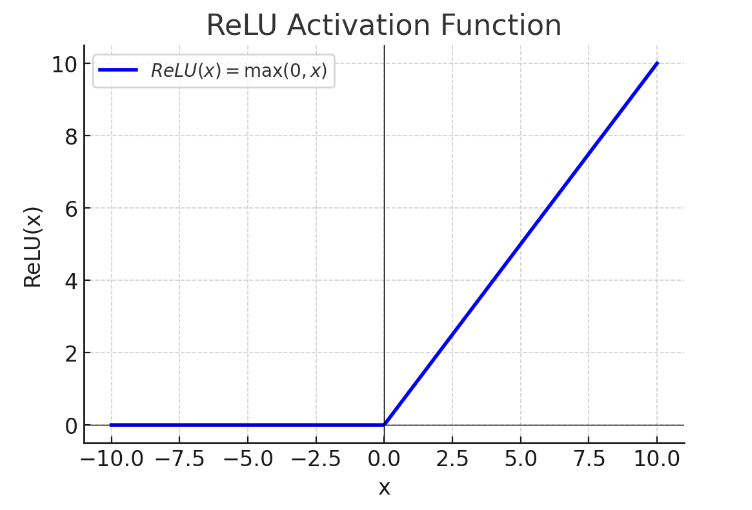
When the data is less than or equal to 0, we take 0; when it is greater than 0, we keep the original value. This behavior can:
- Make the output of the convolutional layer sparser, with many values becoming 0, reducing redundant information so that the subsequent pooling layer focuses only on meaningful activations
- Suppress noise and reduce interference from negative values, making the model more stable
At this point, you might ask: the logic that ReLU can perform can also be done by Sigmoid, so why not use Sigmoid? The reason is to prevent vanishing gradients: • Sigmoid: when $x \to +\infty$ or $x \to -\infty$, the gradient approaches 0, making vanishing gradients likely • ReLU: as long as $x > 0$, the gradient is 1, which keeps gradients flowing
2.1.8. Two Major Characteristics of Convolutional Neural Networks
- Parameter sharing: the same feature filter can be applied to the entire image
- Sparsity of connections: each node in the generated feature map is connected only to specific nodes in the original image
2.2. Convolutional Neural Network (CNN) Model Theory (Advanced) - Image Padding, LeNet, and AlexNet
This article follows directly from the previous article, 2.1. Convolutional Neural Network (CNN) Model Theory (Basic) - Convolution, Pooling, and ReLU Function, so if you have not read it yet, it is recommended to read that first.
2.2.1. Image Padding
Convolution introduces two problems:
- The image gets compressed, causing information loss: the convolved image is smaller than the original image
- Edge information is used less and is easier to ignore: center pixels are repeatedly computed during convolution, while edge pixels are computed only once
To address these problems, we use image padding: by adding pixels around the edges of the image, we can keep the image the same size after convolution. The amount of padding is determined by the filter size and the stride, so that the convolved image has the same size as the original image.
- The added pixels are 0, so they do not affect the original image information.
For example, suppose I have a 5×5 image, the filter size is 3×3, and the stride is $(1,1)$. How many pixels should I pad?
The output size is calculated using the following formula: $$ O = \frac{(I - K + 2P)}{S} + 1 $$
Where:
- I is the input size (5×5)
- K is the filter size (3×3)
- P is the padding amount on each side (top/bottom or left/right); the formula uses $2P$ because both sides are padded
- S is the stride (1×1)
If we want the output size to still be $5 \times 5$, we set $O = 5$ and $K = 3$, then solve the equation: $$ 5 = \frac{(5 - 3 + 2P)}{1} + 1 $$ We get $P = 1$. That is, we pad 1 pixel on each side, so the total padding along one dimension is $2P = 2$.
If the required total padding along one dimension is odd, it cannot be split evenly across the two sides, so we need to decide which side gets one extra pixel. A common practice is to pad one extra pixel on the right/bottom, because some deep learning frameworks, such as TensorFlow, default to a “more padding on the bottom/right” strategy.
2.2.2. Classic CNN Models
In the previous article (2.1. Convolutional Neural Network (CNN) Model Theory (Basic) - Convolution, Pooling, and ReLU Function), we mentioned that CNN is a model formed by connecting the following operations:
- Convolution
- Pooling
- MLP
So what is the exact order? Are there steps that need to be repeated? To answer these questions, let us look at what CNN models created by earlier researchers look like.
LeNet-5
LeNet-5 is a classic convolutional neural network (CNN) architecture proposed by Yann LeCun and others in 1998, mainly for handwritten digit recognition, such as on the MNIST dataset.

Input Layer
- Size: $32 \times 32$ grayscale image (the original MNIST size is $28 \times 28$, which is padded to $32 \times 32$)
- Channels: 1 (grayscale image)
First layer: Convolutional Layer C1
- Input size: $32 \times 32 \times 1$
- Filters (kernel): 6 $5 \times 5$ convolution kernels (stride=1, valid padding)
- Computation formula:
$O = \frac{(I - K + 2P)}{S} + 1 = \frac{(32 - 5 + 0)}{1} + 1 = 28$
- Output size: $28 \times 28 \times 6$ (6 feature maps)
- Activation function: Sigmoid (modern CNNs may use ReLU)
Second layer: Pooling Layer S2 (Subsampling / Pooling Layer)
-
Input size: $28 \times 28 \times 6$
-
Operation: $2 \times 2$ average pooling (stride=2)
-
Computation formula: $O = \frac{(I - K)}{S} + 1 = \frac{(28 - 2)}{2} + 1 = 14$
-
Output size: $14 \times 14 \times 6$ (reduced size after pooling)
-
Activation function: Sigmoid
Third layer: Convolutional Layer C3
-
Input size: $14 \times 14 \times 6$
-
Filters: 16 $5 \times 5$ filters
-
Computation formula: $O = \frac{(I - K + 2P)}{S} + 1 = \frac{(14 - 5 + 0)}{1} + 1 = 10$
-
Output size: $10 \times 10 \times 16$
-
Activation function: Sigmoid
-
Connection pattern: not fully connected; only some feature maps are connected, which reduces parameters
Fourth layer: Pooling Layer S4 (Subsampling / Pooling Layer)
-
Input size: $10 \times 10 \times 16$
-
Operation: $2 \times 2$ average pooling (stride=2)
-
Computation formula: $O = \frac{(10 - 2)}{2} + 1 = 5$
-
Output size: $5 \times 5 \times 16$
-
Activation function: Sigmoid
Fifth layer: Fully Connected Layer C5
- Input size: $5 \times 5 \times 16 = 400$ neurons
- Output neurons: 120 (fully connected)
- Activation function: Sigmoid
Sixth layer: Fully Connected Layer F6
- Input neurons: 120
- Output neurons: 84
- Activation function: Sigmoid
Output Layer
- Input neurons: 84
- Output neurons: 10 (corresponding to digits 0-9)
- Activation function: Softmax (for classification tasks)
Let us summarize it in a table:
| Layer | Description | Input Size | Output Size | Kernel Size | Activation |
|---|---|---|---|---|---|
| Input Layer | Grayscale image | $32 \times 32 \times 1$ | $32 \times 32 \times 1$ | - | - |
| C1 Convolution | 6 $5 \times 5$ filters | $32 \times 32 \times 1$ | $28 \times 28 \times 6$ | $5 \times 5$ | Sigmoid |
| S2 Pooling | Average pooling $2 \times 2$ | $28 \times 28 \times 6$ | $14 \times 14 \times 6$ | $2 \times 2$ | Sigmoid |
| C3 Convolution | 16 $5 \times 5$ filters | $14 \times 14 \times 6$ | $10 \times 10 \times 16$ | $5 \times 5$ | Sigmoid |
| S4 Pooling | Average pooling $2 \times 2$ | $10 \times 10 \times 16$ | $5 \times 5 \times 16$ | $2 \times 2$ | Sigmoid |
| C5 Fully Connected | 400 input neurons | $5 \times 5 \times 16 = 400$ | 120 | - | Sigmoid |
| F6 Fully Connected | 120 input neurons | 120 | 84 | - | Sigmoid |
| Output Layer | Softmax classification | 84 | 10 | - | Softmax |
Input image: 32×32 grayscale image, 1 channel Trainable parameters: about 60,000 Features:
- As the network gets deeper, the image height and width shrink while the number of channels increases
- Convolution and pooling are used in pairs, block by block
AlexNet
As science and technology advanced, computer computing power and mathematical theory also developed. LeNet has already been superseded, and its successor is AlexNet.
AlexNet was proposed by Alex Krizhevsky and others in 2012 and achieved great success in the ImageNet competition (ILSVRC-2012). It is considered a milestone in modern deep learning. Compared with LeNet-5, it is deeper and wider, and introduces new techniques such as the ReLU activation function, overlapping pooling, Dropout, and data augmentation, which greatly improved CNN performance on large-scale datasets.
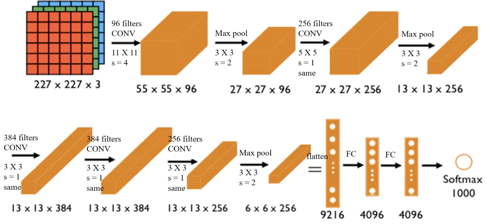
Input Layer
- Size: $227 \times 227 \times 3$ (RGB image)
- Preprocessing: subtract mean for normalization
First layer: Convolutional Layer Conv1
-
Input size: $227 \times 227 \times 3$
-
Filters (kernel): 96 $11 \times 11$ filters, stride S = 4
-
Padding: 0 (valid)
-
Computation formula: $O = \frac{(I - K + 2P)}{S} + 1 = \frac{(227 - 11 + 0)}{4} + 1 = 55$
-
Output size: $55 \times 55 \times 96$
-
Activation function: ReLU
-
Characteristics:
- Large $11 \times 11$ convolution kernels with stride 4 accelerate feature extraction
- ReLU replaces Sigmoid, speeding up convergence
- Local Response Normalization (LRN): enhances contrast
Second layer: Max Pooling Layer Pool1
-
Input size: $55 \times 55 \times 96$
-
Pooling method: $3 \times 3$ max pooling, stride 2
-
Computation formula: $O = \frac{(55 - 3)}{2} + 1 = 27$
-
Output size: $27 \times 27 \times 96$
Third layer: Convolutional Layer Conv2
-
Input size: $27 \times 27 \times 96$
-
Filters: 256 $5 \times 5$ filters, stride 1, padding 2
-
Computation formula: $O = \frac{(27 - 5 + 2 \times 2)}{1} + 1 = 27$
-
Output size: $27 \times 27 \times 256$
-
Activation function: ReLU
-
LRN normalization
-
Characteristics:
- Smaller $5 \times 5$ convolution kernels capture more fine-grained features
- Normalization improves generalization
Fourth layer: Max Pooling Layer Pool2
-
Input size: $27 \times 27 \times 256$
-
Pooling method: $3 \times 3$ max pooling, stride 2
-
Computation formula: $O = \frac{(27 - 3)}{2} + 1 = 13$
-
Output size: $13 \times 13 \times 256$
Fifth layer: Convolutional Layer Conv3
-
Input size: $13 \times 13 \times 256$
-
Filters: 384 $3 \times 3$ filters, stride 1, padding 1
-
Computation formula: $O = \frac{(13 - 3 + 2 \times 1)}{1} + 1 = 13$
-
Output size: $13 \times 13 \times 384$
-
Activation function: ReLU
-
Characteristics: further extracts higher-level features
Sixth layer: Convolutional Layer Conv4
-
Input size: $13 \times 13 \times 384$
-
Filters: 384 $3 \times 3$ filters, stride 1, padding 1
-
Computation formula: $O = 13$
-
Output size: $13 \times 13 \times 384$
-
Activation function: ReLU
-
Characteristics: continues feature extraction and improves hierarchical information
Seventh layer: Convolutional Layer Conv5
-
Input size: $13 \times 13 \times 384$
-
Filters: 256 $3 \times 3$ filters, stride 1, padding 1
-
Computation formula: $O = 13$
-
Output size: $13 \times 13 \times 256$
-
Activation function: ReLU
Eighth layer: Max Pooling Layer Pool3
-
Input size: $13 \times 13 \times 256$
-
Pooling method: $3 \times 3$ max pooling, stride 2
-
Computation formula: $O = \frac{(13 - 3)}{2} + 1 = 6$
-
Output size: $6 \times 6 \times 256$
Ninth layer: Fully Connected Layer FC6
-
Input: $6 \times 6 \times 256 = 9216$ neurons
-
Output: 4096 neurons
-
Activation function: ReLU
-
Characteristics: Dropout (0.5) prevents overfitting
Tenth layer: Fully Connected Layer FC7
-
Input: 4096 neurons
-
Output: 4096 neurons
-
Activation function: ReLU
-
Characteristics: Dropout (0.5)
Eleventh layer: Output Layer (FC8 + Softmax)
- Input: 4096 neurons
- Output: 1000 classes (ImageNet dataset)
- Activation function: Softmax
Summary table:
| Layer | Description | Input Size | Output Size | Filters | Stride | Padding | Activation |
|---|---|---|---|---|---|---|---|
| Input Layer | RGB image | $227 \times 227 \times 3$ | $227 \times 227 \times 3$ | - | - | - | - |
| Conv1 | $11 \times 11$ convolution | $227 \times 227 \times 3$ | $55 \times 55 \times 96$ | $11 \times 11$ | 4 | 0 | ReLU |
| Pool1 | Max pooling | $55 \times 55 \times 96$ | $27 \times 27 \times 96$ | $3 \times 3$ | 2 | - | - |
| Conv2 | $5 \times 5$ convolution | $27 \times 27 \times 96$ | $27 \times 27 \times 256$ | $5 \times 5$ | 1 | 2 | ReLU |
| Pool2 | Max pooling | $27 \times 27 \times 256$ | $13 \times 13 \times 256$ | $3 \times 3$ | 2 | - | - |
(The remaining layers are similar.)
Input image: $227 \times 227 \times 3$ RGB image, 3 channels Trainable parameters: about 60,000,000 (already pretrained and can be used directly)
Features:
- Suitable for recognizing more complex color images, capable of recognizing 1000 classes
- The structure is more complex than LeNet and uses ReLU as the activation function
VGG-16
VGG-16 (Visual Geometry Group 16-layer) was proposed by the VGG group at the University of Oxford in 2014 and achieved excellent results in the ImageNet competition. Its core features are:
- All convolution kernels are $3 \times 3$, which increases depth while reducing parameter count.
- Repeated use of small $3 \times 3$ convolution kernels (2 to 3 convolutions in a block) instead of large kernels such as $5 \times 5$ or $7 \times 7$, improving representational power.
- ReLU is used as the activation function, speeding up training and alleviating the vanishing-gradient problem.
- Dropout is used in the fully connected layers for regularization to reduce overfitting.
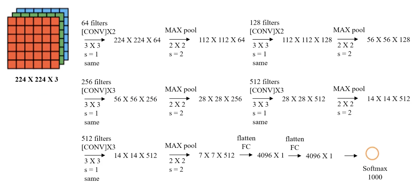
Input Layer
- Size: $224 \times 224 \times 3$ (RGB image)
- Preprocessing:
- Normalization
- Mean subtraction (mean of the ImageNet dataset)
Convolution Block 1 (Conv Block 1)
- Input size: $224 \times 224 \times 3$
- Conv1-1: $3 \times 3$ convolution, 64 filters, stride 1, padding 1
- Conv1-2: $3 \times 3$ convolution, 64 filters, stride 1, padding 1
- Pooling layer (Max Pooling): $2 \times 2$, stride 2
Calculation: $\frac{224 - 3 + 2}{1} + 1 = 224$ $\frac{224 - 2}{2} + 1 = 112$
- Output size: $112 \times 112 \times 64$
Convolution Block 2 (Conv Block 2)
- Input size: $112 \times 112 \times 64$
- Conv2-1: $3 \times 3$ convolution, 128 filters
- Conv2-2: $3 \times 3$ convolution, 128 filters
- Pooling layer: $2 \times 2$, stride 2
- Output size: $56 \times 56 \times 128$
Convolution Block 3 (Conv Block 3)
- Input size: $56 \times 56 \times 128$
- Conv3-1: $3 \times 3$ convolution, 256 filters
- Conv3-2: $3 \times 3$ convolution, 256 filters
- Conv3-3: $3 \times 3$ convolution, 256 filters
- Pooling layer: $2 \times 2$, stride 2
- Output size: $28 \times 28 \times 256$
Convolution Block 4 (Conv Block 4)
- Input size: $28 \times 28 \times 256$
- Conv4-1: $3 \times 3$ convolution, 512 filters
- Conv4-2: $3 \times 3$ convolution, 512 filters
- Conv4-3: $3 \times 3$ convolution, 512 filters
- Pooling layer: $2 \times 2$, stride 2
- Output size: $14 \times 14 \times 512$
Convolution Block 5 (Conv Block 5)
- Input size: $14 \times 14 \times 512$
- Conv5-1: $3 \times 3$ convolution, 512 filters
- Conv5-2: $3 \times 3$ convolution, 512 filters
- Conv5-3: $3 \times 3$ convolution, 512 filters
- Pooling layer: $2 \times 2$, stride 2
- Output size: $7 \times 7 \times 512$
Fully Connected Layers
-
FC1
- Input size: $7 \times 7 \times 512 = 25088$
- Number of neurons: 4096
- Activation function: ReLU
- Dropout: 0.5
-
FC2
- Input size: 4096
- Number of neurons: 4096
- Activation function: ReLU
- Dropout: 0.5
-
Output layer (FC3 + Softmax)
- Input size: 4096
- Output size: 1000 (ImageNet classification)
- Activation function: Softmax
Summary table:
| Layer | Description | Input Size | Output Size | Filters | Stride | Padding | Activation |
|---|---|---|---|---|---|---|---|
| Input Layer | RGB image | $224 \times 224 \times 3$ | $224 \times 224 \times 3$ | - | - | - | - |
| Conv1-1 | $3 \times 3$ convolution | $224 \times 224 \times 3$ | $224 \times 224 \times 64$ | 64 | 1 | 1 | ReLU |
| Conv1-2 | $3 \times 3$ convolution | $224 \times 224 \times 64$ | $224 \times 224 \times 64$ | 64 | 1 | 1 | ReLU |
| Pool1 | Max pooling | $224 \times 224 \times 64$ | $112 \times 112 \times 64$ | $2 \times 2$ | 2 | 0 | - |
| Conv2-1 | $3 \times 3$ convolution | $112 \times 112 \times 64$ | $112 \times 112 \times 128$ | 128 | 1 | 1 | ReLU |
| Conv2-2 | $3 \times 3$ convolution | $112 \times 112 \times 128$ | $112 \times 112 \times 128$ | 128 | 1 | 1 | ReLU |
| Pool2 | Max pooling | $112 \times 112 \times 128$ | $56 \times 56 \times 128$ | $2 \times 2$ | 2 | 0 | - |
(The remaining layers are similar.)
Input image: $224 \times 224 \times 3$ RGB image, 3 channels Trainable parameters: about 138,000,000
Features:
- All convolution filters are 3×3 with stride 1 and padding 1 (“same” convolution), keeping the spatial size unchanged after each convolution
- All pooling layers use 2×2 filters with stride 2
- Compared with AlexNet, it uses more filters to extract contour information and achieves higher accuracy
Using Classic CNN Models for New Scenarios
How do we use these classic CNN models, which have already been proven to perform very well, for new scenarios?
-
Use the structure of a classic CNN model for image preprocessing, then build an MLP model (the most common approach):
- Load a classic CNN model, strip off its FC layers, and preprocess the images
- Use the preprocessed data as input, take the classification result as output, and build an MLP model
- Train the model
-
Build a new model by referring to the classic CNN structure: From the two models described above, we can see that putting convolution and pooling together generally works quite well, so in a new model we can also combine convolution and pooling. The main issue then becomes how to fine-tune the parameters, such as the filter size.
Let us take the first approach as an example:
Suppose I now need to perform binary classification of cat and dog photos based on the VGG16 model. How would I build the binary classification model?
- Remove the MLP part of the original model
- Keep the part of VGG16 that extracts image features
- Train my own MLP model
2.3. Convolutional Neural Network (CNN) Practice (Basic) - Cat and Dog Photo Binary Classification
This article follows from 2.2. Convolutional Neural Network (CNN) Model Theory (Advanced) - Image Padding, LeNet, and AlexNet, so if you have not read it yet, it is recommended to read that first.
2.3.1. Preparation
Please enter the following command in the terminal to download and install:
pip install keras tensorflow
Our task is binary classification of cats and dogs, so we will use cat and dog photos. Here we use a Kaggle Cats and Dogs Classification Dataset. After downloading, unzip it first. In the train folder, create two folders named cat and dog, put the cat photos into cat, and put the dog photos into dog. The final path should look like this:
.\train
	\train
		\dog
			\dog.0.jpg
			\dog.1.jpg
			\dog.2.jpg
			...
		\cat
			\cat.0.jpg
			\cat.1.jpg
			\cat.2.jpg
			...
Just drag the train folder directly into your Python project folder.
2.3.2. Overall Architecture
The overall CNN model is shown below:
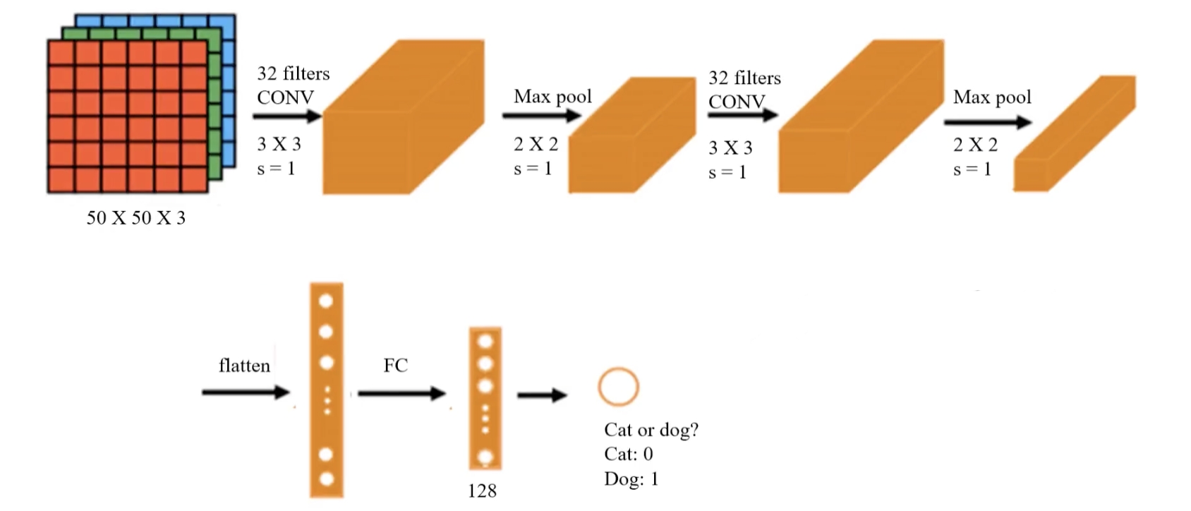
- Input layer:
- The input size is 50 × 50 × 3, meaning the input image is 50×50 pixels with 3 channels (RGB color image).
- First convolution layer (Conv Layer 1):
- Uses 32 3×3 convolution kernels with stride = 1.
- This layer extracts low-level features such as edges and textures.
- The convolution layer uses the ReLU function.
- First pooling layer (Max Pooling 1):
- Pooling kernel size 2×2, stride = 2 (Keras default: stride equals
pool_size). - Max pooling reduces the size of the feature maps, improves computational efficiency, and increases feature robustness.
- Second convolution layer (Conv Layer 2):
- Uses 32 3×3 convolution kernels again, stride = 1.
- Continues to extract higher-level features such as contours and shapes.
- The convolution layer uses the ReLU function.
- Second pooling layer (Max Pooling 2):
- Pooling kernel size 2×2, stride = 2.
- Further reduces the size of the feature maps and reduces computation.
- Flatten layer:
- After two rounds of convolution and pooling, the feature maps are flattened into a one-dimensional vector for input to the fully connected layer.
- Fully connected layer (FC):
- A 128-dimensional fully connected layer is used to learn the final classification decision.
- Output layer:
- The final output is a single neuron, representing the binary classification problem (cat or dog).
- Output 0 means cat, output 1 means dog.
2.3.3. Write the Code
Step 1: Load Images and Preprocess
# Image loading and preprocessing
from keras.preprocessing.image import ImageDataGenerator

train_datagen = ImageDataGenerator(rescale=1./255)
training_set = train_datagen.flow_from_directory('.\\train\\train',
                                                 target_size=(50, 50),
                                                 batch_size=128,
                                                 class_mode='binary')
-
ImageDataGeneratoris a tool for image data augmentation and preprocessing. It can generate richer training data through a series of transformations such as rotation, shifting, and scaling, thereby improving the generalization ability of deep learning models. -
train_datagenis an instance ofImageDataGenerator:rescale=1./255scales the pixel values of the images. Raw pixel values are usually in the range[0, 255]. By setting this parameter, the pixel values are normalized to the[0, 1]range for faster convergence and more stable training.ImageDataGeneratorhas more parameters as well, and can also perform scaling, shifting, rotation, and more.
-
By calling
flow_from_directory(), images are loaded from the specified directory and prepared as a training dataset:- The
target_sizeparameter specifies the target size of the images when they are loaded. This will resize all images to a consistent size, which here is 50×50 pixels. - The
batch_sizeparameter specifies the batch size of images loaded from the generator each time. In deep learning, training data is usually split into several batches, and this parameter defines how many images are included in each batch. Here,batch_size=128means the generator will produce 128 images and their labels at a time. A largerbatch_sizeusually means higher training efficiency. However, if your GPU memory is too small, you can reduce it appropriately (32 is a very good configuration), though that may lead to unstable convergence. - The
class_modeparameter is set to'binary', which means this is a binary classification problem, and the generated labels will be binarized, i.e. 0 or 1. If set to'categorical': used for multi-class problems, labels are one-hot encoded, for example[1, 0, 0]indicates the first class. If set to'sparse': similar to'categorical', but the labels are integer values rather than one-hot vectors, for example0,1,2. If set toNone: no labels are returned, which is usually used for unsupervised learning or prediction (inference) stages.
- The
Note: the path syntax above is for Windows. If you are on macOS/Linux, please use ./train/train.
Step 2: Build the CNN Model
Based on the architecture above, let us build the CNN model:
# Build the model
from keras.models import Sequential
from keras.layers import Conv2D, MaxPooling2D, Flatten, Dense

model = Sequential()
# Convolution layer
model.add(Conv2D(32, (3,3), input_shape=(50,50,3), activation='relu'))
# Pooling layer
model.add(MaxPooling2D(pool_size=(2,2)))
Explanation of the Conv2D parameters:
32 (filters):- Indicates that this layer uses 32 convolution kernels (filters).
- Each kernel extracts different features, so the number of feature maps extracted is the same as the number of kernels. The final output is 32 feature maps.
(3, 3):- Specifies the convolution kernel size as 3x3 pixels (usually a small size such as
(3, 3)or(5, 5)is used). - The convolution kernel slides over the input image to extract local features.
- Specifies the convolution kernel size as 3x3 pixels (usually a small size such as
input_shape=(50,50,3):- Indicates the shape of the input data:
50x50is the image resolution (width, height), and3is the number of channels. Images usually have 3 color channels (RGB). This is the CNN input requirement, so you must make sure the preprocessed image data matches this shape.
- Indicates the shape of the input data:
activation='relu': the activation function is ReLU (Rectified Linear Unit), which turns negative values into 0 and keeps positive values unchanged.
Explanation of the MaxPooling2D parameters:
pool_size=(2,2):- Specifies the pooling window size as 2x2 pixels.
- In each 2x2 window, the maximum value is retained (that is, max pooling), and the other values are discarded.
- Pooling shrinks the image width and height by half. With valid padding, the first convolution layer output size is
48x48, and after pooling it becomes24x24.
At this point we have only written the first convolution + pooling layer. Let us continue with the second convolution + pooling layer:
# Second convolution + pooling layer
model.add(Conv2D(32, (3,3), activation='relu'))
model.add(MaxPooling2D(pool_size=(2,2)))
Conv2Dhere does not need theinput_shapeparameter because the code can infer the output size of the previous layer automatically.
At this point, the feature extraction part of the image is complete. Next, we flatten the features into a one-dimensional vector for the MLP model to consume:
# Flatten layer
model.add(Flatten())
Then we write the MLP architecture (two fully connected layers, with 128 neurons in the hidden layer, and one neuron in the output layer for binary classification):
# Fully connected layer
model.add(Dense(units=128, activation='relu'))
model.add(Dense(units=1, activation='sigmoid'))
Step 3: Train the Model
The next operations are the same as when using only an MLP model: configure the core training parameters:
# Configure training
model.compile(optimizer='adam', loss='binary_crossentropy', metrics=['accuracy'])

# View the model structure
model.summary()
-
compileis a Keras model method used to configure the model’s learning process before training. Its main parameters are:- Loss function (
loss): defines how error is computed during training. - Optimizer (
optimizer): determines how model parameters such as weights and biases are updated to minimize the loss function. - Evaluation metric (
metrics): determines the metric used to evaluate model performance. These metrics do not affect training; they are only used to measure results.
- Loss function (
-
loss='binary_crossentropy':binary_crossentropyis a commonly used loss function for binary classification tasks. -
optimizer='adam':adam(Adaptive Moment Estimation) is an adaptive learning-rate optimization algorithm and one of the most commonly used optimizers in deep learning. -
metrics=['accuracy']: specifies accuracy as the metric used to measure performance during training and evaluation.
Output:
Model: "sequential"
┏━━━━━━━━━━━━━━━━━━━━━━━━━━━━━━━━━┳━━━━━━━━━━━━━━━━━━━━━━━━┳━━━━━━━━━━━━━━━┓
┃ Layer (type)                    ┃ Output Shape           ┃       Param # ┃
┡━━━━━━━━━━━━━━━━━━━━━━━━━━━━━━━━━╇━━━━━━━━━━━━━━━━━━━━━━━━╇━━━━━━━━━━━━━━━┩
│ conv2d (Conv2D)                 │ (None, 48, 48, 32)     │           896 │
├─────────────────────────────────┼────────────────────────┼───────────────┤
│ max_pooling2d (MaxPooling2D)    │ (None, 24, 24, 32)     │             0 │
├─────────────────────────────────┼────────────────────────┼───────────────┤
│ conv2d_1 (Conv2D)               │ (None, 22, 22, 32)     │         9,248 │
├─────────────────────────────────┼────────────────────────┼───────────────┤
│ max_pooling2d_1 (MaxPooling2D)  │ (None, 11, 11, 32)     │             0 │
├─────────────────────────────────┼────────────────────────┼───────────────┤
│ flatten (Flatten)               │ (None, 3872)           │             0 │
├─────────────────────────────────┼────────────────────────┼───────────────┤
│ dense (Dense)                   │ (None, 128)            │       495,744 │
├─────────────────────────────────┼────────────────────────┼───────────────┤
│ dense_1 (Dense)                 │ (None, 1)              │           129 │
└─────────────────────────────────┴────────────────────────┴───────────────┘
 Total params: 506,017 (1.93 MB)
 Trainable params: 506,017 (1.93 MB)
 Non-trainable params: 0 (0.00 B)
Next, feed the data into the model:
# Train the model
model.fit(training_set, epochs=25)
epochsdetermines the number of training iterations.
Step 4: Evaluate the Model
Let us see its prediction accuracy on the training data:
# Calculate the model prediction accuracy
accuracy_train = model.evaluate(x=training_set)
print("\nAccuracy on training set: ", accuracy_train[1])
Output:
Accuracy on training set: 0.9990400075912476
You can see that the accuracy is very high.
2.4. Convolutional Neural Network (CNN) Practice (Advanced) - Using VGG-16 for Image Feature Extraction
This article follows from 2.2. Convolutional Neural Network (CNN) Model Theory (Advanced) - Image Padding, LeNet, and AlexNet, so if you have not read it yet, it is recommended to read that first.
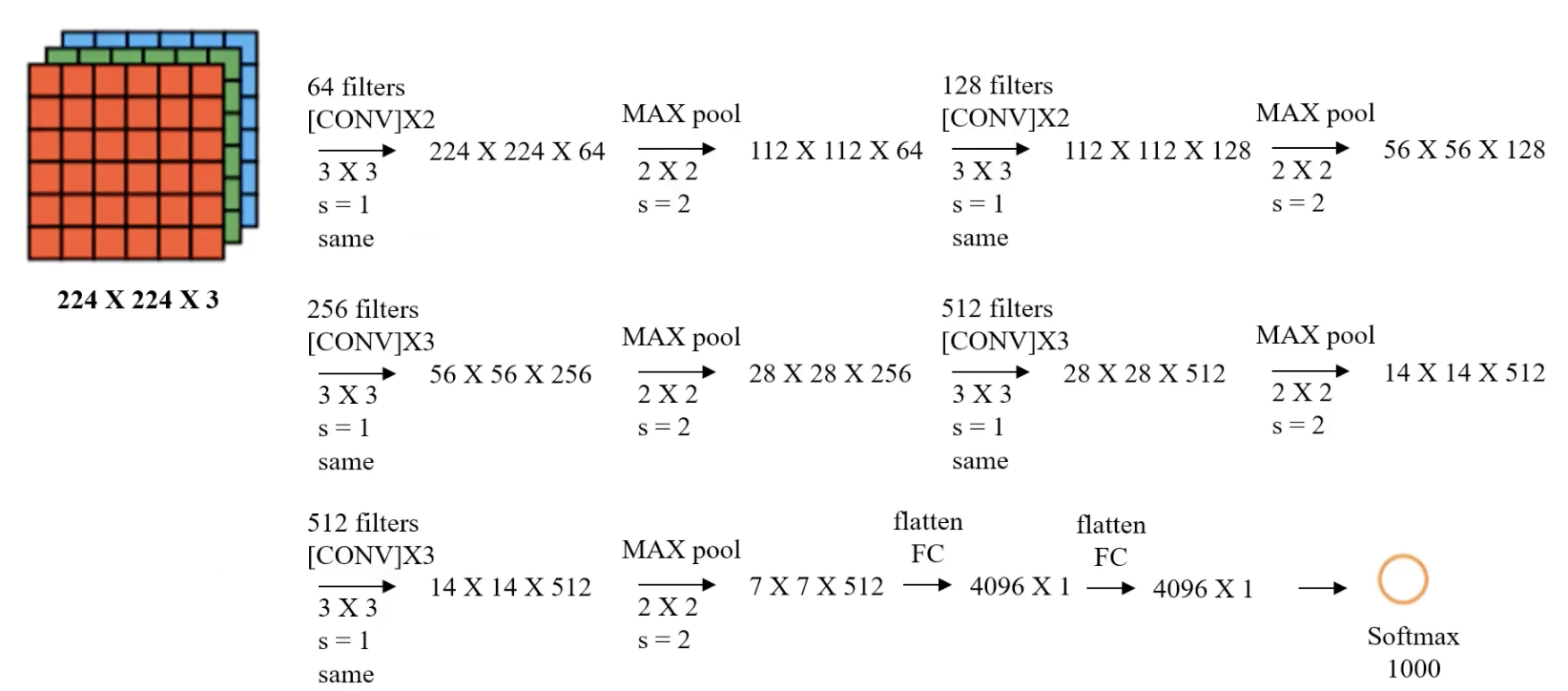
2.4.1. VGG-16 Architecture
In this article, we will use VGG-16 for image feature extraction and then build our own binary classification model. Let us first review the architecture of VGG-16:
| Layer | Description | Input Size | Output Size | Filters | Stride | Padding | Activation |
|---|---|---|---|---|---|---|---|
| Input Layer | RGB image | $224 \times 224 \times 3$ | $224 \times 224 \times 3$ | - | - | - | - |
| Conv1-1 | $3 \times 3$ convolution | $224 \times 224 \times 3$ | $224 \times 224 \times 64$ | 64 | 1 | 1 | ReLU |
| Conv1-2 | $3 \times 3$ convolution | $224 \times 224 \times 64$ | $224 \times 224 \times 64$ | 64 | 1 | 1 | ReLU |
| Pool1 | Max pooling | $224 \times 224 \times 64$ | $112 \times 112 \times 64$ | $2 \times 2$ | 2 | 0 | - |
| Conv2-1 | $3 \times 3$ convolution | $112 \times 112 \times 64$ | $112 \times 112 \times 128$ | 128 | 1 | 1 | ReLU |
| Conv2-2 | $3 \times 3$ convolution | $112 \times 112 \times 128$ | $112 \times 112 \times 128$ | 128 | 1 | 1 | ReLU |
| Pool2 | Max pooling | $112 \times 112 \times 128$ | $56 \times 56 \times 128$ | $2 \times 2$ | 2 | 0 | - |
(The remaining layers are similar.)
After feature extraction, we will build our own MLP model with one hidden layer and 10 neurons.
2.4.2. Preparation
Please enter the following command in the terminal to download and install:
pip install keras tensorflow scikit-learn
Our task is binary classification of cats and dogs, so we will use cat and dog photos. Here we use a Kaggle Cats and Dogs Classification Dataset. After downloading, unzip it first. In the train folder, create two folders named cat and dog, put the cat photos into cat, and put the dog photos into dog. The final path should look like this:
.\train
	\train
		\dog
			\dog.0.jpg
			\dog.1.jpg
			\dog.2.jpg
			...
		\cat
			\cat.0.jpg
			\cat.1.jpg
			\cat.2.jpg
			...
Just drag the train folder directly into your Python project folder.
If you want to work through this project locally, I strongly recommend using a NVIDIA GPU with CUDA acceleration in a Linux environment, or manually enabling ROCm on an AMD GPU (Linux only). You can of course use Windows, but TensorFlow no longer supports GPU acceleration on Windows, so you will have to rely on pure CPU computation, which is much slower. It takes me 10+ minutes on an i9-13900KF and 30 minutes on an M1 Max.
To enable ROCm on an AMD GPU, you need to install the TensorFlow version adapted for ROCm (Linux only), which can be installed directly with pip:
pip install tensorflow-rocm
Run the following code to check whether TensorFlow can detect the AMD GPU:
import tensorflow as tf
print("Num GPUs Available:", len(tf.config.list_physical_devices('GPU')))
2.4.3. Memory-Saving Version
Step 1: Initialize VGG-16
# Initialize the VGG model (remove the fully connected MLP layers)
from tensorflow.keras.applications.vgg16 import VGG16
model = VGG16(weights='imagenet', include_top=False)
weights='imagenet'means the weights loaded are pretrained on the ImageNet datasetinclude_top=False:- Means the top fully connected layers of VGG-16 (the classification part) are not loaded, and only the convolutional part is kept
- The purpose is to use VGG-16 as a feature extractor to extract high-level convolutional features
Step 2: Load Images
# Define a function: load and preprocess a single image
from tensorflow.keras.applications.vgg16 import preprocess_input
import numpy as np
from tensorflow.keras.preprocessing.image import img_to_array, load_img

def load_image_and_preprocess(image_path, model):
    """
    Load an image and preprocess it to fit the VGG model
    :param image_path: image path
    :param model: VGG model instance
    :return: preprocessed feature vector
    """
    img = load_img(image_path, target_size=(224, 224))  # Resize the image
    img = img_to_array(img)  # Convert to array
    x = np.expand_dims(img, axis=0)  # Expand dimensions to match model input format
    x = preprocess_input(x)  # Apply preprocessing (such as mean centering)
    x_vgg = model.predict(x)  # Extract features
    return np.reshape(x_vgg, (7 * 7 * 512))  # Flatten the features

# Define a function: process all images in a single folder
import os

def process_folder(folder, model):
    """
    Process all images in the specified folder and extract feature vectors
    :param folder: image folder path
    :param model: VGG model instance
    :return: extracted feature vector array
    """
    # Get all .jpg file paths
    img_paths = [
        os.path.join(folder, file)
        for file in os.listdir(folder)
        if file.endswith('.jpg')
    ]

    # Initialize the feature array (the shape after feature extraction is 7*7*512)
    features = np.zeros((len(img_paths), 7 * 7 * 512))

    # Iterate over all file paths and load/extract features one by one
    for idx, path in enumerate(img_paths):
        features[idx] = load_image_and_preprocess(path, model)
        print(f"Preprocessed: {path}")

    return features, len(img_paths)

# Process the cat image folder
cat_folder = "train/train/cat"
cat_features, cat_count = process_folder(cat_folder, model)  # Cat features and count

# Process the dog image folder
dog_folder = "train/train/dog"
dog_features, dog_count = process_folder(dog_folder, model)  # Dog features and count
Define the single-image loading and preprocessing function (load_image_and_preprocess):
- Loads the image at the specified path and resizes it to the 224x224 input size required by VGG16.
- Converts the image from PIL format to a NumPy array and expands the dimensions to match the model input format (4D tensor).
- Uses
preprocess_inputto normalize the image data (VGG16 requires a specific input format, such as mean centering). - Calls
model.predictto use the VGG16 model to extract features, producing convolutional feature maps of size (7, 7, 512). - Flattens the feature map into a one-dimensional vector (7×7×512) for later processing.
Define the folder-level image processing function (process_folder):
- Iterates over the specified folder and filters out all image file paths ending in
.jpg. - Initializes an empty feature matrix (
features) with shape (number of images, 7×7×512). - Calls
load_image_and_preprocessfor each image to extract features and stores them in the feature matrix. - Returns the extracted feature matrix and the number of images.
Extract features from the cat and dog image folders:
- Specify the folder paths for cat and dog images (
cat_folderanddog_folder). - Call
process_folderseparately for the two folders to extract a feature vector for each image, returning the feature matrices (cat_featuresanddog_features) and the corresponding image counts (cat_countanddog_count).
Step 3: Generate the Corresponding Labels
We need to provide labels for the training and test data:
# Generate the corresponding labels (cats are 0, dogs are 1)
cat_labels = np.zeros((cat_count, 1))
dog_labels = np.ones((dog_count, 1))

# Merge the cat and dog features and labels
X = np.concatenate((cat_features, dog_features), axis=0)
y = np.concatenate((cat_labels, dog_labels), axis=0)

# Print the result information
print(f"Feature shape: {X.shape}, Label shape: {y.shape}")
Output:
Feature shape: (25000, 25088), Label shape: (25000, 1)
Step 4: Split the Data
We need to split the data into a training set and a test set. The training set is used to train the model, and the test set is used to evaluate model accuracy:
# Split the data
from sklearn.model_selection import train_test_split

X_train, X_test, y_train, y_test = train_test_split(X,
                                                    y,
                                                    test_size=0.2,
                                                    random_state=50)
X: the input feature matrix. Here,Xis the image feature matrix extracted by VGG-16 and flattened into one dimension(None, 7 * 7 * 512). It is the feature set for training and testing.y: the label values, i.e. the category each image belongs to. Here we usey, which represents the labels generated earlier, with cats as 0 and dogs as 1.test_size=0.2: the proportion of the entire dataset used as the test set. Here it is set to 20% (80% for training, 20% for testing).random_state=50: the random seed used to ensure consistent randomness in data splitting. The same seed ensures the training and test sets are the same each time the program runs.
Step 5: Build the MLP Model
Next, we build our own MLP model with one hidden layer, 10 neurons, and one output neuron for binary classification:
# MLP model
from keras.models import Sequential
from keras.layers import Dense
model = Sequential()
model.add(Dense(units=10, activation='relu', input_dim=7 * 7 * 512))
model.add(Dense(units=1, activation='sigmoid'))
Step 6: Configure the Model
# Configure the model
model.compile(optimizer='adam', loss='binary_crossentropy', metrics=['accuracy'])
-
compileis a Keras model method used to configure the model’s learning process before training. Its main parameters are:- Loss function (
loss): defines how error is computed during training. - Optimizer (
optimizer): determines how model parameters such as weights and biases are updated to minimize the loss function. - Evaluation metric (
metrics): determines the metric used to evaluate model performance. These metrics do not affect training; they are only used to measure results.
- Loss function (
-
loss='binary_crossentropy':binary_crossentropyis a commonly used loss function for binary classification tasks. -
optimizer='adam':adam(Adaptive Moment Estimation) is an adaptive learning-rate optimization algorithm and one of the most commonly used optimizers in deep learning. -
metrics=['accuracy']: specifies accuracy as the metric used to measure performance during training and evaluation.
Step 7: Train the Model
Feed the training set data into the model:
# Train the model
model.fit(X_train, y_train, epochs=50)
Step 8: Evaluate the Model
We need to test the accuracy on the training set and the test set separately:
# Training set accuracy
train_accuracy = model.evaluate(X_train, y_train)[1]
print('Train Accuracy: ', train_accuracy)

# Test set accuracy
test_accuracy = model.evaluate(X_test, y_test)[1]
print('Test Accuracy: ', test_accuracy)
Output:
Train Accuracy:  0.9991000294685364
Test Accuracy:  0.9833999872207642
The result is very good!
2.4.4. Higher-Efficiency Version
In the section above, we processed the photos one by one. The advantage of this approach is that it does not consume much memory, but the efficiency is lower. We can also load all photos into memory at once and process them together, which is more efficient.
In actual tests, loading all photos into memory at once will use 20GB of memory, and with the IDE included (I use PyCharm Professional), the total memory usage is about 23GB. In other words, you need 32GB of memory to run it barely, and 48GB to make sure you do not run out of memory.
If your computer has enough memory, you can try the following code:
import os
import numpy as np
from tensorflow.keras.preprocessing.image import load_img, img_to_array
from tensorflow.keras.applications.vgg16 import VGG16, preprocess_input

# Initialize the VGG model
model = VGG16(weights='imagenet', include_top=False)

def load_and_preprocess_images(folder):
    """
    Batch load and preprocess all images in the specified folder
    :param folder: image folder path
    :return: preprocessed batch image data and image count
    """
    # Check whether the path exists
    if not os.path.exists(folder):
        raise FileNotFoundError(f"Folder does not exist: {folder}")

    # Get all .jpg file paths
    img_paths = [
        os.path.join(folder, file)
        for file in os.listdir(folder)
        if file.endswith('.jpg')
    ]

    if not img_paths:
        raise ValueError(f"No image files found in folder: {folder}")

    # Load all images in batch and resize them to (224, 224)
    images = np.array([
        img_to_array(load_img(img_path, target_size=(224, 224)))
        for img_path in img_paths
    ])

    # Apply preprocessing (such as mean centering)
    images = preprocess_input(images)

    print(f"Loaded {len(images)} images from {folder}")
    return images, len(img_paths)

def process_folder_in_batch(folder, model):
    """
    Batch process all images in the specified folder and extract feature vectors
    :param folder: image folder path
    :param model: VGG model instance
    :return: extracted feature vector array and image count
    """
    # Load and preprocess all images
    images, img_count = load_and_preprocess_images(folder)

    # Extract feature vectors in batch
    features = model.predict(images)
    features = features.reshape(img_count, -1)  # Flatten to a (N, 7*7*512) feature matrix

    print(f"Extracted features for {img_count} images from {folder}")
    return features, img_count

# Paths
BASE_DIR = os.path.abspath("train/train")
cat_folder = os.path.join(BASE_DIR, "cat")
dog_folder = os.path.join(BASE_DIR, "dog")

# Process the cat image folder
try:
    cat_features, cat_count = process_folder_in_batch(cat_folder, model)
except Exception as e:
    print(f"An error occurred while processing the cat image folder: {e}")

# Process the dog image folder
try:
    dog_features, dog_count = process_folder_in_batch(dog_folder, model)
except Exception as e:
    print(f"An error occurred while processing the dog image folder: {e}")

# Check whether feature extraction succeeded
if 'cat_features' in locals() and 'dog_features' in locals():
    # Generate the corresponding labels (cats are 0, dogs are 1)
    cat_labels = np.zeros((cat_count, 1))
    dog_labels = np.ones((dog_count, 1))

    # Merge features and labels
    X = np.concatenate((cat_features, dog_features), axis=0)
    y = np.concatenate((cat_labels, dog_labels), axis=0)

    print(f"Feature shape: {X.shape}, Label shape: {y.shape}")

    # Split the data
    from sklearn.model_selection import train_test_split

    X_train, X_test, y_train, y_test = train_test_split(X, y, test_size=0.2, random_state=50)
else:
    print("Feature extraction failed, so subsequent processing cannot continue.")

# Build the MLP model
from tensorflow.keras.models import Sequential
from tensorflow.keras.layers import Dense
model = Sequential()
model.add(Dense(units=10, activation='relu', input_dim=7 * 7 * 512))
model.add(Dense(units=1, activation='sigmoid'))

# Configure the model
model.compile(optimizer='adam', loss='binary_crossentropy', metrics=['accuracy'])

# Train the model
model.fit(X_train, y_train, epochs=50)

# Training set accuracy
train_accuracy = model.evaluate(X_train, y_train)[1]
print('Train Accuracy: ', train_accuracy)

# Test set accuracy
test_accuracy = model.evaluate(X_test, y_test)[1]
print('Test Accuracy: ', test_accuracy)
3.1. Sequence Model
3.1.1. Some Examples
Let’s look at some real-world applications of sequence models:
- Automatically writing an article from a title
- Automatically finding names in a sentence
- …
Their common core is making predictions based on text content and the information before and after it.
Let’s look at another example:
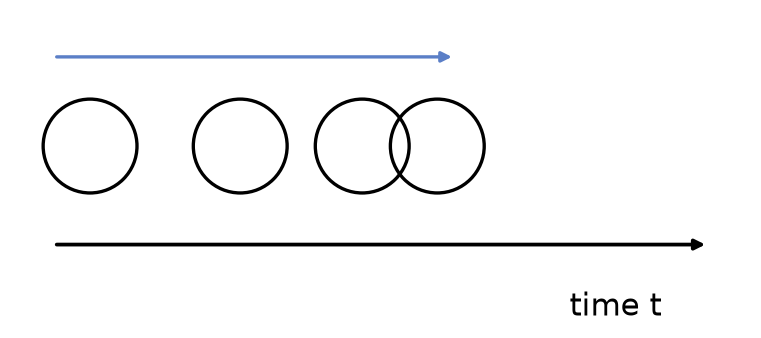
There is a ball moving in one direction, but its speed is not fixed. I want the computer to predict where the ball is at a certain moment. If we had such an algorithm, we could use visual monitoring to anticipate human behavior.
The core of this problem is making predictions based on the object’s state at different moments in time.
Finally, one more example:
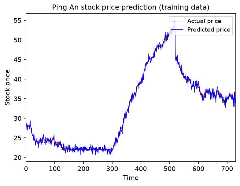
Using historical stock prices to predict tomorrow’s stock price. Although it is impossible to predict it very accurately, as long as the trend is right, it can still help investors make decisions.
The core of this problem is making predictions based on historical data.
These three examples all have one thing in common: they estimate outcomes from sequential data with an order relationship.
This kind of problem can be handled by a sequence model.
3.1.2. What Is a Sequence Model
Sequence models are a class of machine learning models designed specifically to handle time-series data or ordered data. They can capture temporal dependencies in input data and are widely used in natural language processing (NLP), speech recognition, and time-series forecasting.
Common sequence models include:
- RNNs (Recurrent Neural Networks): able to process variable-length input, but they suffer from vanishing gradients.
- LSTMs (Long Short-Term Memory networks) and GRUs (Gated Recurrent Units): improvements over RNNs that capture long-range dependencies better.
- Transformers: based on the self-attention mechanism, they have surpassed RNNs/LSTMs in NLP tasks and have become the mainstream architecture today, such as BERT and GPT.
Their main characteristics are:
- The elements in the input and output sequences have an order. Different orders should produce different results. For example, “not eating” and “eating not” have different meanings.
- The lengths of the input and output can vary. Examples include article generation and chatbots.
Their main application areas are:
- Speech recognition
- Language translation
- Stock price prediction
- Behavior prediction
One fun fact: the Transformer architecture was originally designed for natural language processing (NLP) tasks, especially machine translation. It first appeared in Google’s 2017 paper “Attention Is All You Need”, which completely changed the NLP field.
In the next article, 3.2. Recurrent Neural Network (RNN) Theory (Basic), we will learn about the most widely used sequence model before the Transformer era: the RNN, or recurrent neural network.
3.2. Recurrent Neural Network (RNN) Theory (Basic)
3.2.1. What Is a Recurrent Neural Network (RNN)
A recurrent neural network (RNN) is a neural network used to process sequence data, such as time series, text, and speech. Unlike ordinary feedforward neural networks, RNNs have a kind of “memory” and can retain past information to influence the current output. That makes them very suitable for temporal data and natural language tasks.
To understand RNNs, we first need to review the MLP model. Here is a simplified model:
graph TD;
    X((x)) --> |input| A[computing unit] --> |output| Y((y))
x is taken as input and passed into the computing unit, where several neurons in each layer produce the output y. An RNN, however, feeds the result of the previous computation into the next computation as a new parameter:
graph TD;
    X1((x^1)) --> A1[computing unit]
    A1 --> Y1((y^1))
    A1 -->|a^1| A2[computing unit]
    X2((x^2)) --> A2
    A2 --> Y2((y^2))
- $x^1$ and $x^2$ are inputs at two time steps.
- The computing unit processes the data at each time step and outputs $y^1$ and $y^2$.
- The hidden state $a^1$ is passed across time steps, meaning information from the previous step flows into the next step. The hidden state is computed from the previous hidden state and the current input.
3.2.2. The Mathematical Model of RNNs
Basic Architecture
Let’s look at the basic architecture of an RNN:
graph TD;
    A0((a^0)) --> A1[computing unit]
    X1((x^1)) --> A1
    A1 --> Y1((y^1))
    A1 --> Y2((a^1))
$a^0$: Initial Hidden State
- This is the initial value of the hidden state at the first time step.
- It is usually set to a zero vector (all zeros), or it can be randomly initialized: $a^0 = \mathbf{0} \quad \text{(default)}$
- Purpose: provide an initial memory so that the RNN has temporal characteristics.
$x^1$: Input at the First Time Step
- The sequence input processed by the RNN, namely the data at the first time step.
- It may be:
- Text tasks: the first word in a sentence, such as “Hello”
- Time series: the first time point in stock data
- Speech recognition: the first frame of an audio segment
- This input is used together with the hidden state $a^0$ to compute the new hidden state $a^1$.
Computing Unit
- The core unit of an RNN uses the previous hidden state $a^0$ and the current input $x^1$ to compute:
- a new hidden state $a^1$ (memory passing)
- the output at the current time step $y^1$ (prediction)
- Formulas: $$ a^1 = f(W_h a^0 + W_x x^1 + b) $$ $$ y^1 = g(W_y a^1 + c) $$
- $W_h$, $W_x$, and $W_y$ are weight matrices
- $b$ and $c$ are bias terms
- $f$ (commonly
tanh) is the activation function for the hidden state - $g$ (such as
softmax) is the output mapping
This article uses the common form above: first update the hidden state $a^1$, then compute the output $y^1$ from $a^1$. Some materials write an equivalent variant that maps $a^0$ and $x^1$ to $y^1$ in one step; the meaning is the same once the weight matrices are defined consistently.
$y^1$: Output at the First Time Step
- This is the main output of the computing unit, representing the prediction result at the current time step
- For different tasks:
- Language models such as GPT: $y^1$ may be the probability distribution for the next word
- Machine translation: $y^1$ may be the first word in the target language
- Speech recognition: $y^1$ may be a phoneme or a word
- Formula:
$$
y^1 = g(W_y a^1 + c)
$$
- Here, $g$ may be softmax for classification tasks, or linear activation for regression tasks
$a^1$: Updated Hidden State
- The memory information for the next time step, used to carry historical information to $t=2$
- Formula:
$$
a^1 = f(W_h a^0 + W_x x^1 + b)
$$
- This value is passed to the next time step $t=2$ to compute $a^2$ and $y^2$
And So On
The two most important formulas are the ones for the two outputs: $$ a^1 = f(W_h a^0 + W_x x^1 + b) $$ $$ y^1 = g(W_y a^1 + c) $$
- $W_h$, $W_x$, and $W_y$ are weight matrices
- $b$ and $c$ are bias terms
- $f$ (commonly
tanh) is the activation function for the hidden state - $g$ (such as
softmax) is the output mapping
What we need to do is repeat this process over and over: $$ a^i = f(W_h a^{i-1} + W_x x^{i} + b) $$ $$ y^i = g(W_y a^i + c) $$
3.2.3. Computers and RNNs
So what do we want the computer to calculate in an RNN model? Looking at the two formulas above, the unknown parameters are the weight matrices $W_h$, $W_x$, and $W_y$.
The method for computing these parameters is the same as in MLPs: use training data and labels to backpropagate gradients, and find the weight matrices $W_h$, $W_x$, and $W_y$ that minimize the loss function.
3.2.4. Example
Let’s use an example to deepen our understanding of RNNs:
Automatically find the names in a sentence: GTC is hosted by Jensen Huang.
First, let’s define our inputs—each word (including punctuation) corresponds to one input data point:
| Input | Word |
|---|---|
| $x_1$ | “GTC” |
| $x_2$ | “is” |
| $x_3$ | “hosted” |
| $x_4$ | “by” |
| $x_5$ | “Jensen” |
| $x_6$ | “Huang” |
| $x_7$ | “.” |
How should the labels be written? Each input corresponds to one output. Since we want to find names, inputs that are part of a name are 1, and the rest are 0:
| Input | Word | Output |
|---|---|---|
| $x_1$ | “GTC” | 0 |
| $x_2$ | “is” | 0 |
| $x_3$ | “hosted” | 0 |
| $x_4$ | “by” | 0 |
| $x_5$ | “Jensen” | 1 |
| $x_6$ | “Huang” | 1 |
| $x_7$ | “.” | 0 |
But computers do not understand words directly; what they see are encodings. So we need to convert words into a form that the computer can understand—numbers. In other words, we build a dictionary that maps input words to numerical vectors and convert each input word into the corresponding dictionary value.
How should we build this dictionary? The simplest and most direct way is to create a dictionary that covers all words, and the two case variants of the same first letter should be treated as separate entries: $$ \left{ \begin{array}{ll} \textit{a} & : 1 \ \textit{am} & : 2 \ \vdots & \vdots \ \textit{by} & : x \ \vdots & \vdots \ \textit{is} & : y \ \textit{hosted} & : z \ \vdots & \vdots \end{array} \right} $$
We use the one-hot encoding corresponding to each word as input. For example, the word am would be represented as:
| Index | Value |
|---|---|
| 0 | 0 |
| 1 | 1 |
| 2 | 0 |
| 3 | 0 |
| 4 | 0 |
| 5 | 0 |
| … | 0 |
How do we build the model?
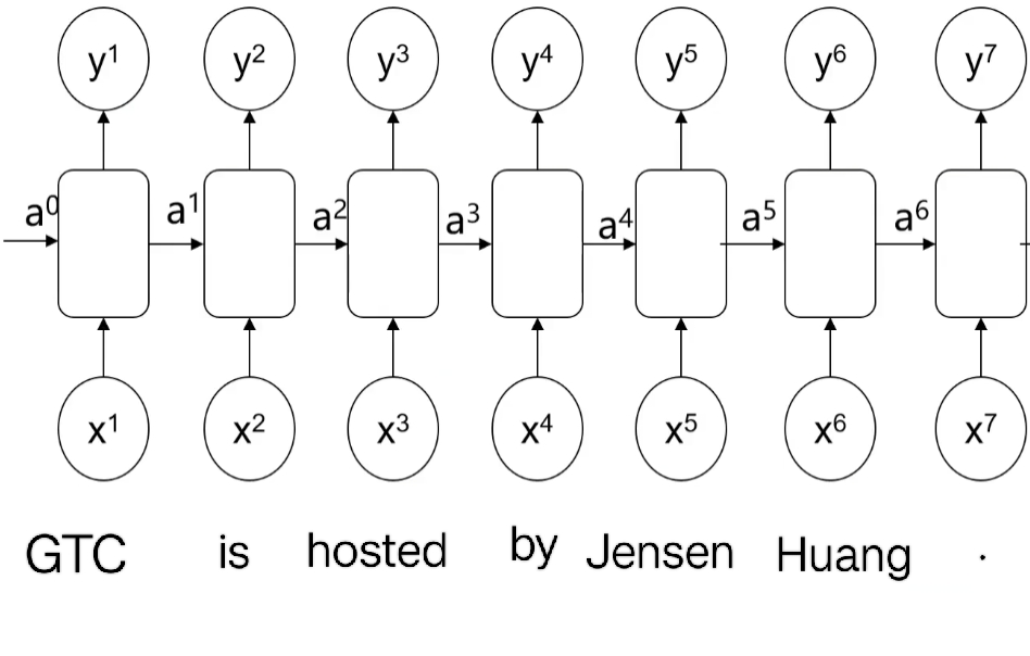
Seven inputs correspond to seven time steps (the same RNN cell and weights are reused at each step). Feed the one-hot encoded data and the corresponding labels to the model, and let the model back-calculate the weights.
When the computer back-calculates the weights, it needs to ensure that the loss function is minimized. The loss function for a single neuron is: $$ \textit{loss}(i) = -y^i \log(y_{\textit{predict}}^i) - (1 - y^i) \log(1 - y_{\textit{predict}}^i) $$ We add together the loss functions of all neurons and let the computer minimize the total in each iteration: $$ \operatorname{minimize}( \sum_{i} \left[ -y^i \log(y_{\textit{predict}}^i) - (1 - y^i) \log(1 - y_{\textit{predict}}^i) \right]) $$
If you do not want to build a dictionary containing every English word, you can also build a dictionary for each character: $$ \left{ \begin{array}{ll} \textit{a} & : 1 \ \textit{b} & : 2 \ \vdots & \vdots \ \textit{z} & : 26 \ \textit{A} & : 27 \ \vdots & \vdots \ \textit{1} & : 53 \ \vdots & \vdots \end{array} \right} $$ This makes the dictionary smaller, but it places higher demands on the model.
3.3. Recurrent Neural Network (RNN) Theory (Advanced)
This article continues from 3.2. Recurrent Neural Network (RNN) Theory (Basic). If you have not read that one yet, it is recommended that you start there.
3.3.1. Basic RNN Structure
Diagram
Let’s first look at the most basic RNN structure:
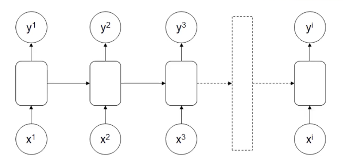
On top of the MLP structure, some information from the earlier sequence is processed and then passed to the next sequence.
Sometimes you may also see this symbol:
This corresponds to the basic RNN structure and can be used to represent an RNN model. Compared with an MLP, it has one extra arrow indicating self-recurrence.
Inputs & Outputs
- Inputs: $x^1, x^2, x^3, \dots, x^i$
- Outputs: $y^1, y^2, y^3, \dots, y^i$
The feature here is that the input and output sequences are the same length: if there are $i$ inputs, there are also $i$ outputs. This is the RNN structure with multiple inputs and multiple outputs of the same dimension.
Main Applications
Recognizing specific information, such as identifying which words in a sentence are names.
3.3.2. RNN Architecture with Multiple Inputs and One Output
Diagram
Inputs & Outputs
- Inputs: $x^1, x^2, x^3, \dots, x^i$
- Output: $y^1$
Main Applications
Sentiment recognition: if I have the sentence “I feel happy and positive.”, the computer needs to determine whether this sentence expresses positive or negative sentiment.
3.3.3. RNN Architecture with One Input and Multiple Outputs
Diagram
Inputs & Outputs
- Input: $x^1$
- Outputs: $y^1, y^2, y^3, \dots, y^i$
It is generally used as a sequence data generator.
Main Applications
- Article generation: given a title, generate a paragraph.
- Music generation: choose parameters such as style or emotion and output music.
3.3.4. RNN Architecture with Multiple Inputs and Multiple Outputs
Diagram
How is this different from the basic RNN architecture? The difference is that the number of input items and output items does not have to be the same.
Inputs & Outputs
- Inputs: $x^1, x^2, x^3, \dots, x^i$
- Outputs: $y^1, y^2, y^3, \dots, y^j$
Main Applications
Its main application is machine translation, although Transformers have now basically replaced RNNs. For example, consider the following sentence: “What is artificial intelligence?” (4 words, not counting punctuation)
The computer translates it into Chinese: “什么是人工智能?” (7 Chinese characters, not counting punctuation)
Here, the number of input and output words is different.
3.3.5. Limitations of the Vanilla RNN Structure
Vanilla RNNs all have structural limitations. As early sequence information is passed to later positions, its weight gradually decreases, which causes important information to be lost.
Let’s look at a simple example (fill in the past tense):
- “The student, who got A+ in the exam, ___ excellent.”
- “The students, who got A+ in the exam, ___ excellent.”
The first sentence clearly takes was because of the keyword “student”, and the second clearly takes were because of the keyword “students”.
However, an RNN loses information at each transfer, so by the end the difference between “student” and “students” may no longer be reflected.
To address this problem, we need to increase the decision weight of important early information.
3.3.6. Introduction to Long Short-Term Memory Networks (LSTM)
Diagram
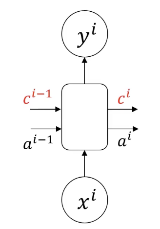
Features
LSTM adds a memory cell $c^i$, which can pass along information from distant earlier positions. For example, the singular/plural difference between “student” and “students” in the example above can be stored in the memory cell.
In simpler terms: compared with $a^i$, the memory cell $c^i$ focuses on recording important early sequence information, and it loses less information during transfer.
3.3.7. A Deeper Look at LSTM
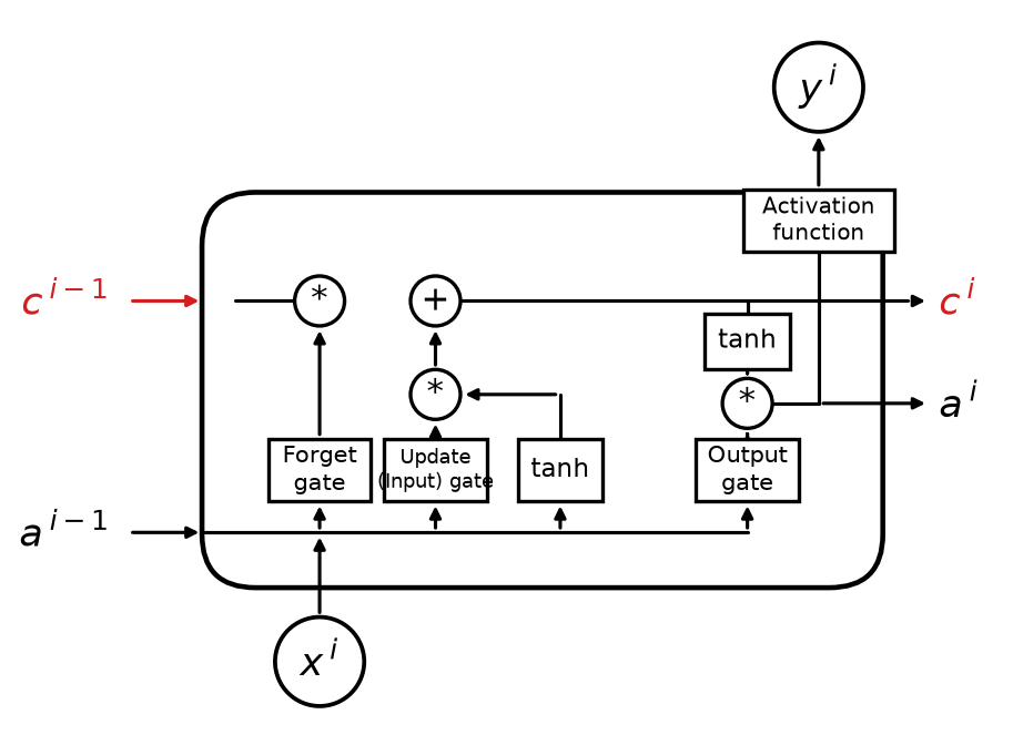
1. Inputs and outputs
-
Inputs: The inputs of this LSTM unit include:
-
The current input $x^i$
-
The previous hidden state $a^{i-1}$
-
The previous cell state $c^{i-1}$ (marked in red)
-
Outputs:
- The current hidden state $a^i$
- The current cell state $c^i$ (marked in red)
- The output $y^i$ after the activation function
2. Key computation units The key components of LSTM are the forget gate, input gate, output gate, and a new way of computing the cell state:
(1) Forget Gate
- Role: decide which information should be forgotten from the previous cell state $c^{i-1}$.
- Computation:
$$
f^i = \sigma(W_f [a^{i-1}, x^i] + b_f)
$$
- Here, $\sigma$ is the sigmoid activation function
- $W_f$ is the weight matrix and $b_f$ is the bias term
- The resulting $f^i$ lies between 0 and 1 and represents the forgetting ratio
(2) Input Gate
-
Role: decide which new information should be added to the cell state.
-
Computation: $$ g^i = \tanh(W_g [a^{i-1}, x^i] + b_g) $$
- Here, $g^i$ represents new information, also called the candidate cell state, and is normalized with tanh.
-
At the same time, another gating mechanism determines the proportion of information to add: $$ i^i = \sigma(W_i [a^{i-1}, x^i] + b_i) $$
- $i^i$ is also a value produced by sigmoid and represents how much this information affects the new cell state.
Cell state update: $$ c^i = f^i \cdot c^{i-1} + i^i \cdot g^i $$
(3) Output Gate
- Role: decide the value of the current hidden state, that is, $a^i$.
- Computation:
$$
o^i = \sigma(W_o [a^{i-1}, x^i] + b_o)
$$
- Here, $o^i$ controls how much of the state is output.
Compute the final hidden state: $$ a^i = o^i \cdot \tanh(c^i) $$
3. Key connection explanation
- The red $c^i$ and $c^{i-1}$ indicate the transmission of the LSTM cell state
- $a^i$ and $a^{i-1}$ are the hidden-state transfers used at the next time step
- The input $x^i$ passes through multiple gates to control its information flow
- Activation functions such as tanh play a normalization role in the cell state and output gate
3.3.8. Deep Recurrent Neural Networks (DRNN)
To solve more complex sequence tasks, you can stack single-layer RNNs or combine them with an ordinary MLP structure before the output:
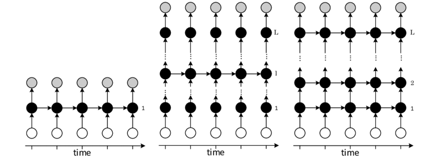
1. Left: Single-layer RNN
- This is the most basic RNN structure. The input depends on the time step, and the hidden layer propagates information through time
- Black nodes indicate hidden states, and arrows indicate the direction of information flow
- Because it only has one hidden layer, this structure has limitations when modeling complex sequences
2. Middle: Multi-layer RNN
- This structure preserves the RNN property along the time dimension while stacking multiple hidden layers along the depth dimension
- The hidden state of a lower layer is not only connected to the next time step, but is also passed upward as input to the next hidden layer, allowing the model to learn representations at different levels (lower layers learn local patterns, higher layers learn long-term dependencies)
- This gives the model greater expressive power and enables it to extract more complex features
3. Right: Fully Connected Deep RNN
- This structure further strengthens the network’s modeling capability. The hidden state of each layer is connected to the next layer and also propagated across time steps
- Such a structure can better capture long-term dependencies while using depth to improve feature learning
Key features of DRNN
- Deep structure: compared with a single-layer RNN, a DRNN has multiple hidden layers, allowing the model to learn different feature representations at different levels and improving expressiveness
- Stronger feature learning: stacking layers helps the network learn hierarchical temporal features. Vanishing gradients along time and depth can still occur, so LSTM/GRU cells or residual connections are often used in practice
- Hierarchical information flow: information is propagated across different time steps and different layers, improving prediction capability
We will take a deeper look at this in the practical section later.
3.4. Recurrent Neural Network (RNN) In Practice - Predicting Stock Prices
This article continues from 3.2. Recurrent Neural Network (RNN) Theory (Basic). If you have not read that one yet, it is recommended that you start there.
3.4.1. Preparation
Please run the following command in your terminal to install the required packages:
pip install keras tensorflow pandas
This article uses my csv file, which I uploaded to GitHub. Click the link to view and download it.
It contains two columns of information: one column is Time, representing time points from 1 to 700, for a total of 700 points; one column is Value, representing the stock price.
Just place the downloaded data in your Python project.
3.4.2. Model Details
Before we start coding, let’s first settle a few model details:
- A single-layer RNN with 5 neurons in the output, and then one final output determined from the values of those 5 neurons
- Use the first eight data points each time to predict the ninth data point
3.4.3. Coding It Up
Step 1: Read the Data
Use the pandas library to read the data and assign variables at the same time:
# Load the data
import pandas as pd
data = pd.read_csv('simulated_stock_data.csv')

prices = data.loc[:, 'Value']
times = data.loc[:, 'Time']
Then use matplotlib to plot the raw data:
# Visualize the raw data
import matplotlib.pyplot as plt
plt.plot(times, prices)
plt.show()
Image output:
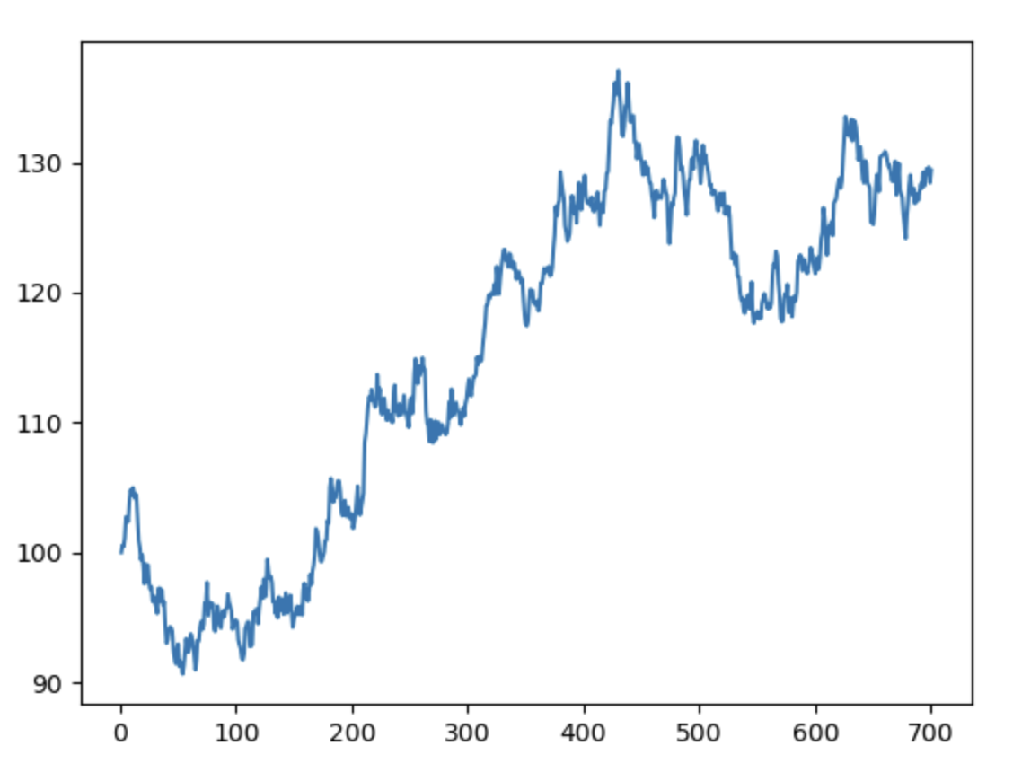
Step 2: Normalize the Data
From the plot above, we can see that our data ranges from around 90 to around 130. The gap is too large, and it is easy to end up with a situation like a steep bowl with a flat bottom. To avoid this, we normalize the data by dividing by the maximum price, so values fall in $(0, 1]$ and gradient descent sees a smoother contour.
# Normalize the data
price_norm = prices / max(prices)
Step 3: Extract X and y
As mentioned above, we use the first eight data points to predict the ninth point, so we need to extract the sequence data first. Every eight data points form a group, and these groups are stacked into a 2D array:
# Extract X and y
import numpy as np
def extract_xy(data, time_step):
    X, y = [], []
    for i in range(len(data) - time_step):
        X.append([a for a in data[i: i + time_step]])
        y.append(data[i + time_step])
    X = np.array(X)
    X = np.reshape(X, (X.shape[0], X.shape[1], 1))
    return X, y

time_step = 8
X, y = extract_xy(price_norm, time_step)
-
time_stepindicates how many consecutive data points are used as one input group to predict the next point. Heretime_step = 8, so each input contains 8 values. -
The loop runs from
0tolen(data) - time_stepto ensure it stays within array bounds. In each iteration:data[i: i + time_step]extracts the consecutivetime_stepdata points starting at positioni(that is, 8 points) and stores them inXdata[i + time_step]extracts the value at positioni + time_stepas the target and stores it iny- For example: if
data = [1, 2, 3, 4, 5, 6, 7, 8, 9]andtime_step = 3, after running the loop we getX = [[1, 2, 3], [2, 3, 4], [3, 4, 5], [4, 5, 6], [5, 6, 7], [6, 7, 8]]andy = [4, 5, 6, 7, 8, 9]
-
Finally, we use NumPy to reshape
X:- For
X, reshape it to(samples, time_step, 1). Each sample represents a group oftime_stepvalues, and we add an extra dimension for the deep-learning model input, representing the number of features, which is 1 here - For
y, keep it as a one-dimensional sequence of lengthsamples(one target per input window). Keras accepts this format for a single regression output
- For
Step 4: Build and Configure the Model
Now we can build the RNN model. Remember to follow the requirements above: a single-layer RNN, 5 neurons in the output, and then one final output determined from the values of those 5 neurons:
# Build the model
from tensorflow.keras.models import Sequential
from tensorflow.keras.layers import Dense, SimpleRNN

model = Sequential()
model.add(SimpleRNN(units=5, input_shape=(time_step, 1), activation='relu'))
model.add(Dense(units=1, activation='linear'))
model.compile(loss='mean_squared_error', optimizer='adam')
model.summary()
-
SimpleRNN layer:
units=5: defines the output dimension of the RNN as 5, which is the size of the hidden state in this layerinput_shape=(time_step, 1):time_step=8(defined in the previous code): indicates that the input has 8 time steps1: indicates that the dimensionality of each time step is 1, because the normalized input is a scalar stock-price value and has only one column
activation='relu': uses the ReLU activation function to encourage nonlinear modeling
-
Dense layer:
units=1: defines the output dimension as 1, used to predict a single price valueactivation='linear': uses a linear activation so that the output is directly a numerical value, in the form of linear regression
-
Compile the model:
loss='mean_squared_error': uses mean squared error as the loss function, which is suitable for regression problemsoptimizer='adam': Adam optimizer, an optimization algorithm that combines momentum and adaptive learning-rate adjustment
-
Print the model architecture:
model.summary()prints a summary of the model structure, including the name of each layer, output dimensions, and parameter counts
Output:
Model: "sequential"
┏━━━━━━━━━━━━━━━━━━━━━━━━━━━━━━━━━┳━━━━━━━━━━━━━━━━━━━━━━━━┳━━━━━━━━━━━━━━━┓
┃ Layer (type)                    ┃ Output Shape           ┃       Param # ┃
┡━━━━━━━━━━━━━━━━━━━━━━━━━━━━━━━━━╇━━━━━━━━━━━━━━━━━━━━━━━━╇━━━━━━━━━━━━━━━┩
│ simple_rnn (SimpleRNN)          │ (None, 5)              │            35 │
├─────────────────────────────────┼────────────────────────┼───────────────┤
│ dense (Dense)                   │ (None, 1)              │             6 │
└─────────────────────────────────┴────────────────────────┴───────────────┘
 Total params: 41 (164.00 B)
 Trainable params: 41 (164.00 B)
 Non-trainable params: 0 (0.00 B)
Step 5: Train the Model
Just feed the data to the model:
# Train the model
model.fit(X, y, epochs=200, batch_size=32)
Step 6: Training-Set Predictions
Finally, let’s look at the model’s predictions and overlay them on the original data to see how large the difference is:
# Training-set prediction
y_train_predict = model.predict(X) * max(prices)
y_train = [i*max(prices) for i in y]

import matplotlib.pyplot as plt
plt.plot(y_train, label='real_price')
plt.plot(y_train_predict, label='predict_price')
plt.legend()
plt.show()
* max(prices):- converts the predicted values back to their original scale
max(prices)is the maximum value used during normalization, and now it is used to map the prediction results back to the actual price range
Image output:
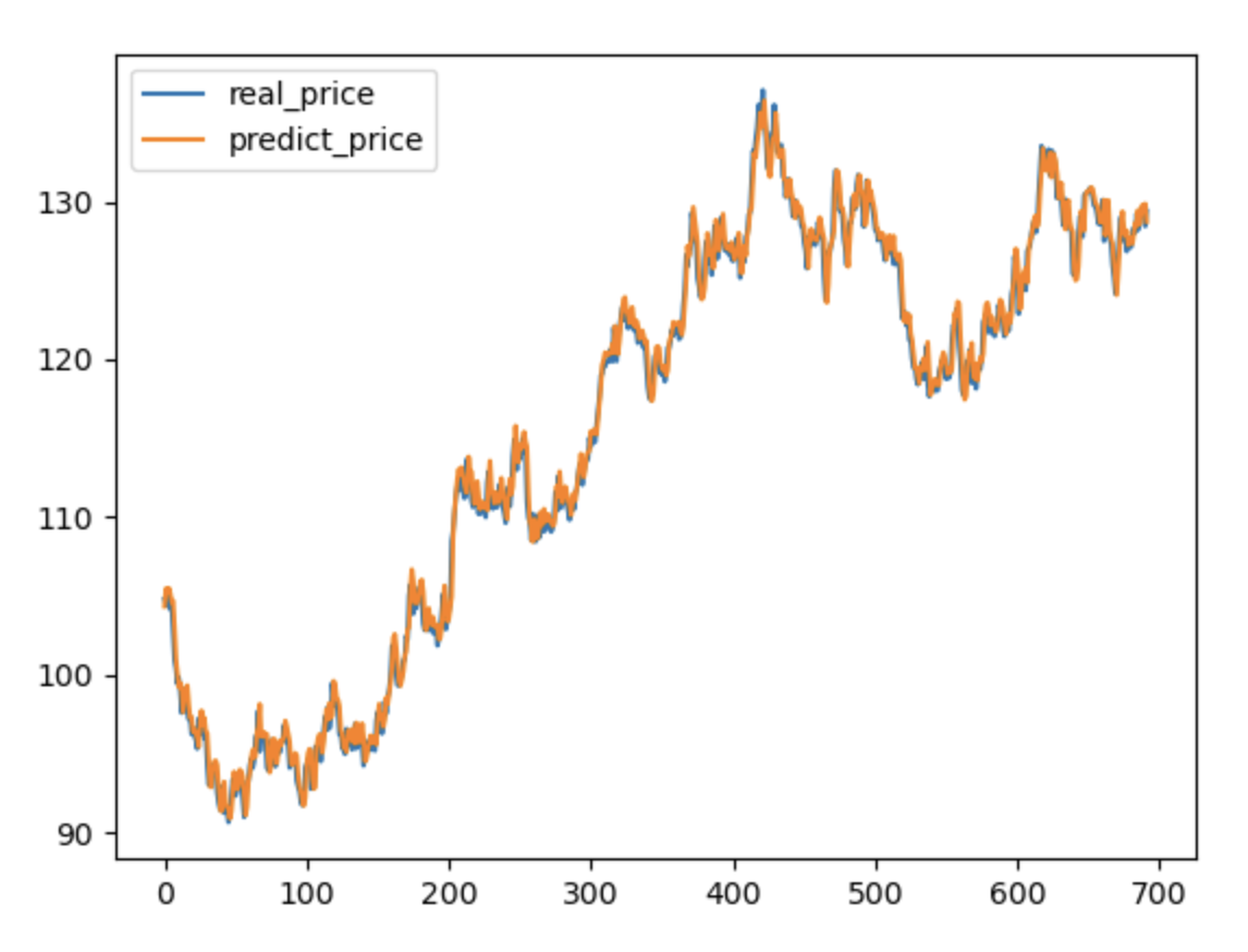
You can see that the result is pretty good, and the gap is not large.
3.5. Recurrent Neural Network (RNN) In Practice - LSTM Text Generation
This article continues from 3.3. Recurrent Neural Network (RNN) Theory (Advanced). If you have not read that one yet, it is recommended that you start there.
3.5.1. Preparation
Please run the following command in your terminal to install the required packages:
pip install keras tensorflow scikit-learn
This article uses my txt file, which I uploaded to GitHub. Click the link to view and download it. We use Mary Shelley’s Frankenstein as the training data.
Just place the downloaded data in your Python project.
3.5.2. Model Architecture
In this article we will use a Long Short-Term Memory (LSTM) model for text generation. We will feed the model the dictionary obtained after converting the text, then let it predict the 21st character from the first 20 characters and calculate accuracy.
Each input sample is a sequence of 20 time steps (characters). The LSTM layer has 20 units, and the number of neurons in the output layer depends on how many different characters appear in the text.
3.5.3. Coding It Up
Step 1: Load the Data
First, we load the data and remove line breaks at the same time:
# Load the data
data = open('Frankenstein_by_Mary_Shelley.txt').read()

# Remove line breaks
data = data.replace('\n', ' ').replace('\r', '')
Step 2: Build the Dictionary
Each character in the text needs its own entry in the dictionary. First we remove duplicate characters and then build the dictionary:
# Remove duplicate characters
letters = list(set(data))

# Print for checking
print(len(letters))

# Build the dictionary
char_to_int = {b:a for a, b in enumerate(letters)}
-
By using
set(data), we remove duplicates from all characters in the text and keep one unique copy of each character, such as letters, numbers, punctuation marks, and so on.list(set(data))turns those unique characters into a list and stores them in the variableletters. -
The dictionary
char_to_intuses the corresponding character as the key and an integer starting from 0 as the value, so that characters can be converted to numeric data and then to one-hot format.
Output:
74
These 74 different characters (uppercase and lowercase letters, digits, punctuation, and so on) make up the entire text.
Step 3: Input Processing
Next we need to process the string in batches. Here we first define a data_processing method, and later we can call it to extract the X and y data the model can receive:
# Batch processing of characters
import numpy as np
from tensorflow.keras.utils import to_categorical

# Implement batch processing for character-based text input: the full text, sliding-window size, and conversion dictionary
def data_processing(data, slide, num_letters, char_to_int):
    # Extract data with a sliding window
    def extract_data(data, slide):
        x = []
        y = []
        for i in range(len(data) - slide):
            x.append([a for a in data[i:i + slide]])
            y.append(data[i + slide])
        return x, y

    # Convert characters to integers in batches
    def char_to_int_data(x, y, char_to_int):
        x_to_int = []
        y_to_int = []
        for i in range(len(x)):
            x_to_int.append([char_to_int[char] for char in x[i]])
            y_to_int.append([char_to_int[char] for char in y[i]])
        return x_to_int, y_to_int

    char_data = extract_data(data, slide)
    int_data = char_to_int_data(char_data[0], char_data[1], char_to_int)
    Input = int_data[0]
    Output = list(np.array(int_data[1]).flatten())
    Input_Reshaped = np.array(Input).reshape(len(Input), slide)
    new_ = np.zeros((Input_Reshaped.shape[0], Input_Reshaped.shape[1], num_letters))
    for i in range(Input_Reshaped.shape[0]):
        for j in range(Input_Reshaped.shape[1]):
            new_[i, j, :] = to_categorical(Input_Reshaped[i, j], num_letters)
    return new_, Output
extract_data function:
- Purpose: extract samples from the input character sequence using a sliding window.
x: the list of characters inside the window (length = window size).y: the target character immediately following the window (the prediction target).
- Logic:
xis obtained with[a for a in data[i:i + slide]], which takes the characters within the current window range.ytakes the first character after the window,data[i + slide].- Example: if
slide=3anddata="abcdefg", the result is:x = [['a', 'b', 'c'], ['b', 'c', 'd'], ['c', 'd', 'e'], ['d', 'e', 'f']]y = ['d', 'e', 'f', 'g']
char_to_int_data function:
- Purpose: convert the character sequences
xand target charactersyinto integer sequences.- It uses the
char_to_intdictionary to get the integer index of each character. - Example: if the input is
x = [['a', 'b', 'c'], ['b', 'c', 'd']],y = ['d', 'e'], and the dictionary is{'a': 0, 'b': 1, 'c': 2, 'd': 3, 'e': 4}, the result is:x_to_int = [[0, 1, 2], [1, 2, 3]]y_to_int = [[3], [4]](later flattened to[3, 4]inOutput)
- It uses the
Conversion to model input:
- Through
extract_dataandchar_to_int_data, we extract the data and convert characters to integers; - The original integer input
Inputhas shape[number of samples, window size]; Outputis the target character sequence, stored as a one-dimensional array.
One-hot encoding processing:
- Purpose: convert the integer input
Input_Reshapedinto a 3D one-hot inputnew_.Input_Reshaped[i, j]is the integer value of thejth character in theith sample of the window.to_categorical(Input_Reshaped[i, j], num_letters)builds the one-hot encoding of the character with dimension[num_letters].- The encoding result of each sample is stored in
new_, whose shape is[number of samples, window size, number of characters].
Final output:
new_: one-hot encoded input array with shape[number of samples, window size, vocabulary size], suitable for deep-learning models such as LSTMs.Output: integer array of target sequences, one-dimensional, with length equal to the number of samples.
Step 4: Get the Model Input
We now use the data_processing method to extract the X and y data the model can receive, while also confirming that the time step is 20 (the model predicts the next character based on the previous 20 characters):
# Time step
time_step = 20

# Get the model input data
X, y = data_processing(data, time_step, len(letters), char_to_int)

# Check the data structure
print(X.shape)
print(len(y))
Output:
(421397, 20, 74)
421397
-
(421397, 20, 74):421397: the number of samples extracted by the sliding window, that is, how many[input sequence -> target character]samples were built. This depends on the relationship between the text lengthlen(data)and the sliding-window sizetime_step.20: the number of time steps per sample, i.e. the sliding-window sizetime_step, which means each input sequence contains 20 characters. This value is determined bytime_step = 20in the code.74: the number of character categories, i.e. the one-hot encoding dimension. This comes from the vocabulary sizelen(letters), meaning there are 74 unique characters in the input data, including letters, punctuation, spaces, and so on.
-
yis the list of target-character integers for the samples. Each sample has one target character, so the length ofyis the same as the number of samples, namely421397.
Step 5: Split the Data
Split the data into training and test sets:
# Split the data
from sklearn.model_selection import train_test_split
X_train, X_test, y_train, y_test = train_test_split(X, y, test_size=0.1, random_state=10)

# Convert y_train to one-hot encoding
y_train_category = to_categorical(y_train, num_classes=len(letters))
- The main reason for converting
y_traininto one-hot encoding is so it can be used to train the LSTM model
Step 6: Build the Model
The model takes sequences of 20 time steps; the LSTM has 20 units, and the number of neurons in the output layer depends on the number of different characters in the text, that is, the length of the dictionary:
# Build the model
from tensorflow.keras.models import Sequential
from tensorflow.keras.layers import Dense, LSTM

model = Sequential()

model.add(LSTM(units=20, input_shape=(time_step, len(letters)), activation='relu'))
model.add(Dense(len(letters), activation='softmax'))
Step 7: Configure the Model
# Configure the model
model.compile(loss='categorical_crossentropy', optimizer='adam', metrics=['accuracy'])
Step 8: Train the Model
Just feed the training data to the model:
# Train the model
model.fit(X_train, y_train_category, epochs=20, batch_size=1000)
batch_size=1000:
- The number of samples used in each training step (gradient update).
- The data will be split into multiple batches, each containing
1000samples.- For example, if there are 50,000 training samples and each batch is 1,000, then 50 updates are needed in one epoch.
- Of course, if you have a lot of memory, you do not need to set this parameter and can load everything into memory at once, although it would take a terrifying 15 GB or so, not even counting the IDE.
Step 9: Evaluate the Model
We evaluate the model using accuracy:
# Training-set accuracy
_, train_accuracy = model.evaluate(X_train, y_train_category)
print(f"Train Accuracy: {train_accuracy}")

# Test-set accuracy
y_test_category = to_categorical(y_test, num_classes=len(letters))
_, test_accuracy = model.evaluate(X_test, y_test_category)
print(f"Test Accuracy: {test_accuracy}")
Output:
Train Accuracy: 0.4766451120376587
Test Accuracy: 0.4727812111377716
Even though this accuracy is still below 50%, keep in mind that the computer has to guess one answer out of 74 different characters, and this result is already quite good. Random guessing would give only 1/74, or 1.35%, so the model’s accuracy is more than 30 times higher.
You can try to improve accuracy further by using a larger LSTM, stacking layers, training longer, or sampling from the predicted distribution to generate longer text.