2.4. Convolutional Neural Network (CNN) Practice (Advanced) - Using VGG-16 for Image Feature Extraction
This article follows from 2.2. Convolutional Neural Network (CNN) Model Theory (Advanced) - Image Padding, LeNet, and AlexNet, so if you have not read it yet, it is recommended to read that first.
2.4.1. VGG-16 Architecture
In this article, we will use VGG-16 for image feature extraction and then build our own binary classification model. Let us first review the architecture of VGG-16:
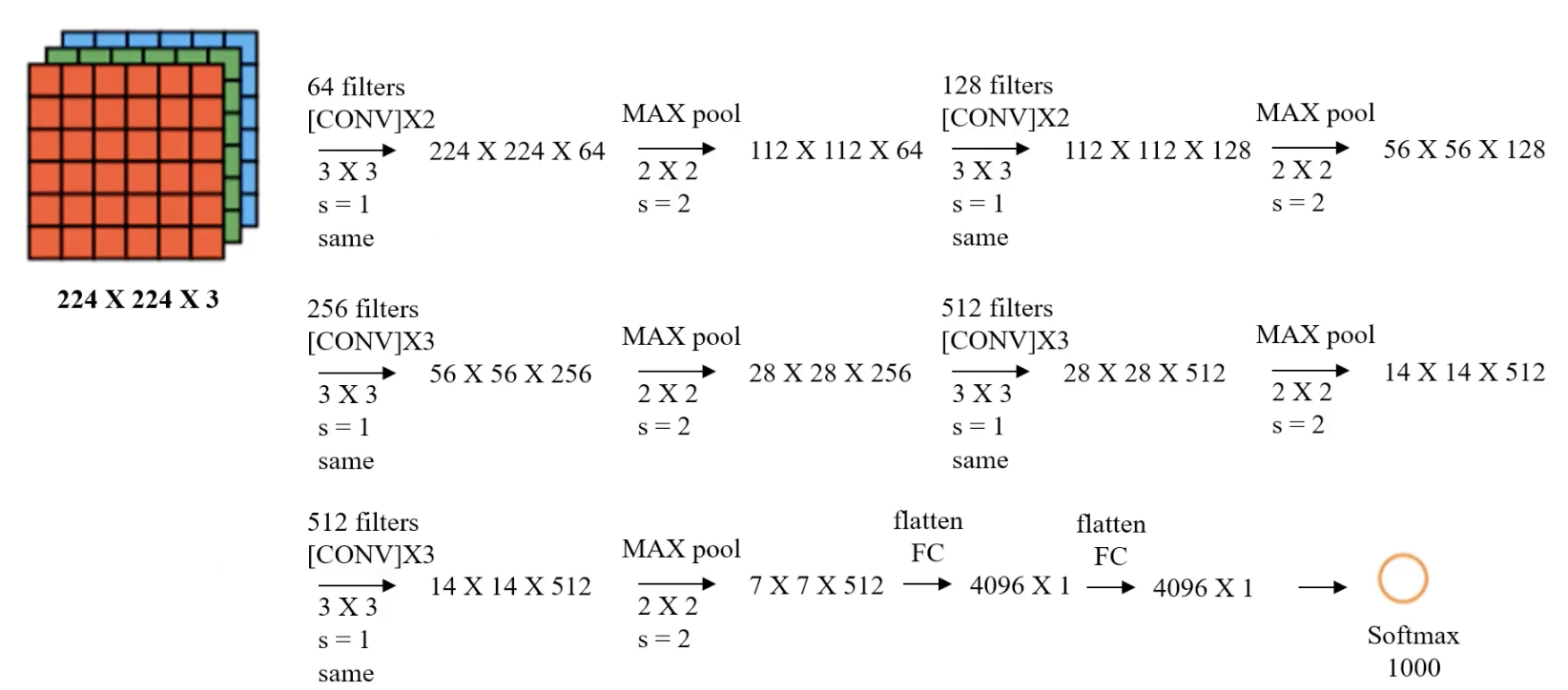
| Layer | Description | Input Size | Output Size | Filters | Stride | Padding | Activation |
|---|---|---|---|---|---|---|---|
| Input Layer | RGB image | $224 \times 224 \times 3$ | $224 \times 224 \times 3$ | - | - | - | - |
| Conv1-1 | $3 \times 3$ convolution | $224 \times 224 \times 3$ | $224 \times 224 \times 64$ | 64 | 1 | 1 | ReLU |
| Conv1-2 | $3 \times 3$ convolution | $224 \times 224 \times 64$ | $224 \times 224 \times 64$ | 64 | 1 | 1 | ReLU |
| Pool1 | Max pooling | $224 \times 224 \times 64$ | $112 \times 112 \times 64$ | $2 \times 2$ | 2 | 0 | - |
| Conv2-1 | $3 \times 3$ convolution | $112 \times 112 \times 64$ | $112 \times 112 \times 128$ | 128 | 1 | 1 | ReLU |
| Conv2-2 | $3 \times 3$ convolution | $112 \times 112 \times 128$ | $112 \times 112 \times 128$ | 128 | 1 | 1 | ReLU |
| Pool2 | Max pooling | $112 \times 112 \times 128$ | $56 \times 56 \times 128$ | $2 \times 2$ | 2 | 0 | - |
(The remaining layers are similar.)
After feature extraction, we will build our own MLP model with one hidden layer and 10 neurons.
2.4.2. Preparation
Please enter the following command in the terminal to download and install:
pip install keras tensorflow scikit-learn
Our task is binary classification of cats and dogs, so we will use cat and dog photos. Here we use a Kaggle Cats and Dogs Classification Dataset. After downloading, unzip it first. In the train folder, create two folders named cat and dog, put the cat photos into cat, and put the dog photos into dog. The final path should look like this:
.\train
	\train
		\dog
			\dog.0.jpg
			\dog.1.jpg
			\dog.2.jpg
			...
		\cat
			\cat.0.jpg
			\cat.1.jpg
			\cat.2.jpg
			...
Just drag the train folder directly into your Python project folder.
If you want to work through this project locally, I strongly recommend using a NVIDIA GPU with CUDA acceleration in a Linux environment, or manually enabling ROCm on an AMD GPU (Linux only). You can of course use Windows, but TensorFlow no longer supports GPU acceleration on Windows, so you will have to rely on pure CPU computation, which is much slower. It takes me 10+ minutes on an i9-13900KF and 30 minutes on an M1 Max.
To enable ROCm on an AMD GPU, you need to install the TensorFlow version adapted for ROCm (Linux only), which can be installed directly with pip:
pip install tensorflow-rocm
Run the following code to check whether TensorFlow can detect the AMD GPU:
import tensorflow as tf
print("Num GPUs Available:", len(tf.config.list_physical_devices('GPU')))
2.4.3. Memory-Saving Version
Step 1: Initialize VGG-16
# Initialize the VGG model (remove the fully connected MLP layers)
from tensorflow.keras.applications.vgg16 import VGG16
model = VGG16(weights='imagenet', include_top=False)
weights='imagenet'means the weights loaded are pretrained on the ImageNet datasetinclude_top=False:- Means the top fully connected layers of VGG-16 (the classification part) are not loaded, and only the convolutional part is kept
- The purpose is to use VGG-16 as a feature extractor to extract high-level convolutional features
Step 2: Load Images
# Define a function: load and preprocess a single image
from tensorflow.keras.applications.vgg16 import preprocess_input
import numpy as np
from tensorflow.keras.preprocessing.image import img_to_array, load_img

def load_image_and_preprocess(image_path, model):
    """
    Load an image and preprocess it to fit the VGG model
    :param image_path: image path
    :param model: VGG model instance
    :return: preprocessed feature vector
    """
    img = load_img(image_path, target_size=(224, 224))  # Resize the image
    img = img_to_array(img)  # Convert to array
    x = np.expand_dims(img, axis=0)  # Expand dimensions to match model input format
    x = preprocess_input(x)  # Apply preprocessing (such as mean centering)
    x_vgg = model.predict(x)  # Extract features
    return np.reshape(x_vgg, (7 * 7 * 512))  # Flatten the features

# Define a function: process all images in a single folder
import os

def process_folder(folder, model):
    """
    Process all images in the specified folder and extract feature vectors
    :param folder: image folder path
    :param model: VGG model instance
    :return: extracted feature vector array
    """
    # Get all .jpg file paths
    img_paths = [
        os.path.join(folder, file)
        for file in os.listdir(folder)
        if file.endswith('.jpg')
    ]

    # Initialize the feature array (the shape after feature extraction is 7*7*512)
    features = np.zeros((len(img_paths), 7 * 7 * 512))

    # Iterate over all file paths and load/extract features one by one
    for idx, path in enumerate(img_paths):
        features[idx] = load_image_and_preprocess(path, model)
        print(f"Preprocessed: {path}")

    return features, len(img_paths)

# Process the cat image folder
cat_folder = "train/train/cat"
cat_features, cat_count = process_folder(cat_folder, model)  # Cat features and count

# Process the dog image folder
dog_folder = "train/train/dog"
dog_features, dog_count = process_folder(dog_folder, model)  # Dog features and count
Define the single-image loading and preprocessing function (load_image_and_preprocess):
- Loads the image at the specified path and resizes it to the 224x224 input size required by VGG16.
- Converts the image from PIL format to a NumPy array and expands the dimensions to match the model input format (4D tensor).
- Uses
preprocess_inputto normalize the image data (VGG16 requires a specific input format, such as mean centering). - Calls
model.predictto use the VGG16 model to extract features, producing convolutional feature maps of size (7, 7, 512). - Flattens the feature map into a one-dimensional vector (7×7×512) for later processing.
Define the folder-level image processing function (process_folder):
- Iterates over the specified folder and filters out all image file paths ending in
.jpg. - Initializes an empty feature matrix (
features) with shape (number of images, 7×7×512). - Calls
load_image_and_preprocessfor each image to extract features and stores them in the feature matrix. - Returns the extracted feature matrix and the number of images.
Extract features from the cat and dog image folders:
- Specify the folder paths for cat and dog images (
cat_folderanddog_folder). - Call
process_folderseparately for the two folders to extract a feature vector for each image, returning the feature matrices (cat_featuresanddog_features) and the corresponding image counts (cat_countanddog_count).
Step 3: Generate the Corresponding Labels
We need to provide labels for the training and test data:
# Generate the corresponding labels (cats are 0, dogs are 1)
cat_labels = np.zeros((cat_count, 1))
dog_labels = np.ones((dog_count, 1))

# Merge the cat and dog features and labels
X = np.concatenate((cat_features, dog_features), axis=0)
y = np.concatenate((cat_labels, dog_labels), axis=0)

# Print the result information
print(f"Feature shape: {X.shape}, Label shape: {y.shape}")
Output:
Feature shape: (25000, 25088), Label shape: (25000, 1)
Step 4: Split the Data
We need to split the data into a training set and a test set. The training set is used to train the model, and the test set is used to evaluate model accuracy:
# Split the data
from sklearn.model_selection import train_test_split

X_train, X_test, y_train, y_test = train_test_split(X,
                                                    y,
                                                    test_size=0.2,
                                                    random_state=50)
X: the input feature matrix. Here,Xis the image feature matrix extracted by VGG-16 and flattened into one dimension(None, 7 * 7 * 512). It is the feature set for training and testing.y: the label values, i.e. the category each image belongs to. Here we usey, which represents the labels generated earlier, with cats as 0 and dogs as 1.test_size=0.2: the proportion of the entire dataset used as the test set. Here it is set to 20% (80% for training, 20% for testing).random_state=50: the random seed used to ensure consistent randomness in data splitting. The same seed ensures the training and test sets are the same each time the program runs.
Step 5: Build the MLP Model
Next, we build our own MLP model with one hidden layer, 10 neurons, and one output neuron for binary classification:
# MLP model
from keras.models import Sequential
from keras.layers import Dense
model = Sequential()
model.add(Dense(units=10, activation='relu', input_dim=7 * 7 * 512))
model.add(Dense(units=1, activation='sigmoid'))
Step 6: Configure the Model
# Configure the model
model.compile(optimizer='adam', loss='binary_crossentropy', metrics=['accuracy'])
-
compileis a Keras model method used to configure the model’s learning process before training. Its main parameters are:- Loss function (
loss): defines how error is computed during training. - Optimizer (
optimizer): determines how model parameters such as weights and biases are updated to minimize the loss function. - Evaluation metric (
metrics): determines the metric used to evaluate model performance. These metrics do not affect training; they are only used to measure results.
- Loss function (
-
loss='binary_crossentropy':binary_crossentropyis a commonly used loss function for binary classification tasks. -
optimizer='adam':adam(Adaptive Moment Estimation) is an adaptive learning-rate optimization algorithm and one of the most commonly used optimizers in deep learning. -
metrics=['accuracy']: specifies accuracy as the metric used to measure performance during training and evaluation.
Step 7: Train the Model
Feed the training set data into the model:
# Train the model
model.fit(X_train, y_train, epochs=50)
Step 8: Evaluate the Model
We need to test the accuracy on the training set and the test set separately:
# Training set accuracy
train_accuracy = model.evaluate(X_train, y_train)[1]
print('Train Accuracy: ', train_accuracy)

# Test set accuracy
test_accuracy = model.evaluate(X_test, y_test)[1]
print('Test Accuracy: ', test_accuracy)
Output:
Train Accuracy:  0.9991000294685364
Test Accuracy:  0.9833999872207642
The result is very good!
2.4.4. Higher-Efficiency Version
In the section above, we processed the photos one by one. The advantage of this approach is that it does not consume much memory, but the efficiency is lower. We can also load all photos into memory at once and process them together, which is more efficient.
In actual tests, loading all photos into memory at once will use 20GB of memory, and with the IDE included (I use PyCharm Professional), the total memory usage is about 23GB. In other words, you need 32GB of memory to run it barely, and 48GB to make sure you do not run out of memory.
If your computer has enough memory, you can try the following code:
import os
import numpy as np
from tensorflow.keras.preprocessing.image import load_img, img_to_array
from tensorflow.keras.applications.vgg16 import VGG16, preprocess_input

# Initialize the VGG model
model = VGG16(weights='imagenet', include_top=False)

def load_and_preprocess_images(folder):
    """
    Batch load and preprocess all images in the specified folder
    :param folder: image folder path
    :return: preprocessed batch image data and image count
    """
    # Check whether the path exists
    if not os.path.exists(folder):
        raise FileNotFoundError(f"Folder does not exist: {folder}")

    # Get all .jpg file paths
    img_paths = [
        os.path.join(folder, file)
        for file in os.listdir(folder)
        if file.endswith('.jpg')
    ]

    if not img_paths:
        raise ValueError(f"No image files found in folder: {folder}")

    # Load all images in batch and resize them to (224, 224)
    images = np.array([
        img_to_array(load_img(img_path, target_size=(224, 224)))
        for img_path in img_paths
    ])

    # Apply preprocessing (such as mean centering)
    images = preprocess_input(images)

    print(f"Loaded {len(images)} images from {folder}")
    return images, len(img_paths)

def process_folder_in_batch(folder, model):
    """
    Batch process all images in the specified folder and extract feature vectors
    :param folder: image folder path
    :param model: VGG model instance
    :return: extracted feature vector array and image count
    """
    # Load and preprocess all images
    images, img_count = load_and_preprocess_images(folder)

    # Extract feature vectors in batch
    features = model.predict(images)
    features = features.reshape(img_count, -1)  # Flatten to a (N, 7*7*512) feature matrix

    print(f"Extracted features for {img_count} images from {folder}")
    return features, img_count

# Paths
BASE_DIR = os.path.abspath("train/train")
cat_folder = os.path.join(BASE_DIR, "cat")
dog_folder = os.path.join(BASE_DIR, "dog")

# Process the cat image folder
try:
    cat_features, cat_count = process_folder_in_batch(cat_folder, model)
except Exception as e:
    print(f"An error occurred while processing the cat image folder: {e}")

# Process the dog image folder
try:
    dog_features, dog_count = process_folder_in_batch(dog_folder, model)
except Exception as e:
    print(f"An error occurred while processing the dog image folder: {e}")

# Check whether feature extraction succeeded
if 'cat_features' in locals() and 'dog_features' in locals():
    # Generate the corresponding labels (cats are 0, dogs are 1)
    cat_labels = np.zeros((cat_count, 1))
    dog_labels = np.ones((dog_count, 1))

    # Merge features and labels
    X = np.concatenate((cat_features, dog_features), axis=0)
    y = np.concatenate((cat_labels, dog_labels), axis=0)

    print(f"Feature shape: {X.shape}, Label shape: {y.shape}")

    # Split the data
    from sklearn.model_selection import train_test_split

    X_train, X_test, y_train, y_test = train_test_split(X, y, test_size=0.2, random_state=50)
else:
    print("Feature extraction failed, so subsequent processing cannot continue.")

# Build the MLP model
from tensorflow.keras.models import Sequential
from tensorflow.keras.layers import Dense
model = Sequential()
model.add(Dense(units=10, activation='relu', input_dim=7 * 7 * 512))
model.add(Dense(units=1, activation='sigmoid'))

# Configure the model
model.compile(optimizer='adam', loss='binary_crossentropy', metrics=['accuracy'])

# Train the model
model.fit(X_train, y_train, epochs=50)

# Training set accuracy
train_accuracy = model.evaluate(X_train, y_train)[1]
print('Train Accuracy: ', train_accuracy)

# Test set accuracy
test_accuracy = model.evaluate(X_test, y_test)[1]
print('Test Accuracy: ', test_accuracy)