2.3. Convolutional Neural Network (CNN) Practice (Basic) - Cat and Dog Photo Binary Classification
This article follows from 2.2. Convolutional Neural Network (CNN) Model Theory (Advanced) - Image Padding, LeNet, and AlexNet, so if you have not read it yet, it is recommended to read that first.
2.3.1. Preparation
Please enter the following command in the terminal to download and install:
pip install keras tensorflow
Our task is binary classification of cats and dogs, so we will use cat and dog photos. Here we use a Kaggle Cats and Dogs Classification Dataset. After downloading, unzip it first. In the train folder, create two folders named cat and dog, put the cat photos into cat, and put the dog photos into dog. The final path should look like this:
.\train
	\train
		\dog
			\dog.0.jpg
			\dog.1.jpg
			\dog.2.jpg
			...
		\cat
			\cat.0.jpg
			\cat.1.jpg
			\cat.2.jpg
			...
Just drag the train folder directly into your Python project folder.
2.3.2. Overall Architecture
The overall CNN model is shown below:
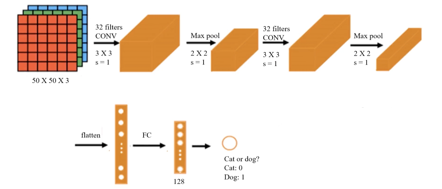
- Input layer:
- The input size is 50 × 50 × 3, meaning the input image is 50×50 pixels with 3 channels (RGB color image).
- First convolution layer (Conv Layer 1):
- Uses 32 3×3 convolution kernels with stride = 1.
- This layer extracts low-level features such as edges and textures.
- The convolution layer uses the ReLU function.
- First pooling layer (Max Pooling 1):
- Pooling kernel size 2×2, stride = 2 (Keras default: stride equals
pool_size). - Max pooling reduces the size of the feature maps, improves computational efficiency, and increases feature robustness.
- Second convolution layer (Conv Layer 2):
- Uses 32 3×3 convolution kernels again, stride = 1.
- Continues to extract higher-level features such as contours and shapes.
- The convolution layer uses the ReLU function.
- Second pooling layer (Max Pooling 2):
- Pooling kernel size 2×2, stride = 2.
- Further reduces the size of the feature maps and reduces computation.
- Flatten layer:
- After two rounds of convolution and pooling, the feature maps are flattened into a one-dimensional vector for input to the fully connected layer.
- Fully connected layer (FC):
- A 128-dimensional fully connected layer is used to learn the final classification decision.
- Output layer:
- The final output is a single neuron, representing the binary classification problem (cat or dog).
- Output 0 means cat, output 1 means dog.
2.3.3. Write the Code
Step 1: Load Images and Preprocess
# Image loading and preprocessing
from keras.preprocessing.image import ImageDataGenerator

train_datagen = ImageDataGenerator(rescale=1./255)
training_set = train_datagen.flow_from_directory('.\\train\\train',
                                                 target_size=(50, 50),
                                                 batch_size=128,
                                                 class_mode='binary')
-
ImageDataGeneratoris a tool for image data augmentation and preprocessing. It can generate richer training data through a series of transformations such as rotation, shifting, and scaling, thereby improving the generalization ability of deep learning models. -
train_datagenis an instance ofImageDataGenerator:rescale=1./255scales the pixel values of the images. Raw pixel values are usually in the range[0, 255]. By setting this parameter, the pixel values are normalized to the[0, 1]range for faster convergence and more stable training.ImageDataGeneratorhas more parameters as well, and can also perform scaling, shifting, rotation, and more.
-
By calling
flow_from_directory(), images are loaded from the specified directory and prepared as a training dataset:- The
target_sizeparameter specifies the target size of the images when they are loaded. This will resize all images to a consistent size, which here is 50×50 pixels. - The
batch_sizeparameter specifies the batch size of images loaded from the generator each time. In deep learning, training data is usually split into several batches, and this parameter defines how many images are included in each batch. Here,batch_size=128means the generator will produce 128 images and their labels at a time. A largerbatch_sizeusually means higher training efficiency. However, if your GPU memory is too small, you can reduce it appropriately (32 is a very good configuration), though that may lead to unstable convergence. - The
class_modeparameter is set to'binary', which means this is a binary classification problem, and the generated labels will be binarized, i.e. 0 or 1. If set to'categorical': used for multi-class problems, labels are one-hot encoded, for example[1, 0, 0]indicates the first class. If set to'sparse': similar to'categorical', but the labels are integer values rather than one-hot vectors, for example0,1,2. If set toNone: no labels are returned, which is usually used for unsupervised learning or prediction (inference) stages.
- The
Note: the path syntax above is for Windows. If you are on macOS/Linux, please use ./train/train.
Step 2: Build the CNN Model
Based on the architecture above, let us build the CNN model:
# Build the model
from keras.models import Sequential
from keras.layers import Conv2D, MaxPooling2D, Flatten, Dense

model = Sequential()
# Convolution layer
model.add(Conv2D(32, (3,3), input_shape=(50,50,3), activation='relu'))
# Pooling layer
model.add(MaxPooling2D(pool_size=(2,2)))
Explanation of the Conv2D parameters:
32 (filters):- Indicates that this layer uses 32 convolution kernels (filters).
- Each kernel extracts different features, so the number of feature maps extracted is the same as the number of kernels. The final output is 32 feature maps.
(3, 3):- Specifies the convolution kernel size as 3x3 pixels (usually a small size such as
(3, 3)or(5, 5)is used). - The convolution kernel slides over the input image to extract local features.
- Specifies the convolution kernel size as 3x3 pixels (usually a small size such as
input_shape=(50,50,3):- Indicates the shape of the input data:
50x50is the image resolution (width, height), and3is the number of channels. Images usually have 3 color channels (RGB). This is the CNN input requirement, so you must make sure the preprocessed image data matches this shape.
- Indicates the shape of the input data:
activation='relu': the activation function is ReLU (Rectified Linear Unit), which turns negative values into 0 and keeps positive values unchanged.
Explanation of the MaxPooling2D parameters:
pool_size=(2,2):- Specifies the pooling window size as 2x2 pixels.
- In each 2x2 window, the maximum value is retained (that is, max pooling), and the other values are discarded.
- Pooling shrinks the image width and height by half. With valid padding, the first convolution layer output size is
48x48, and after pooling it becomes24x24.
At this point we have only written the first convolution + pooling layer. Let us continue with the second convolution + pooling layer:
# Second convolution + pooling layer
model.add(Conv2D(32, (3,3), activation='relu'))
model.add(MaxPooling2D(pool_size=(2,2)))
Conv2Dhere does not need theinput_shapeparameter because the code can infer the output size of the previous layer automatically.
At this point, the feature extraction part of the image is complete. Next, we flatten the features into a one-dimensional vector for the MLP model to consume:
# Flatten layer
model.add(Flatten())
Then we write the MLP architecture (two fully connected layers, with 128 neurons in the hidden layer, and one neuron in the output layer for binary classification):
# Fully connected layer
model.add(Dense(units=128, activation='relu'))
model.add(Dense(units=1, activation='sigmoid'))
Step 3: Train the Model
The next operations are the same as when using only an MLP model: configure the core training parameters:
# Configure training
model.compile(optimizer='adam', loss='binary_crossentropy', metrics=['accuracy'])

# View the model structure
model.summary()
-
compileis a Keras model method used to configure the model’s learning process before training. Its main parameters are:- Loss function (
loss): defines how error is computed during training. - Optimizer (
optimizer): determines how model parameters such as weights and biases are updated to minimize the loss function. - Evaluation metric (
metrics): determines the metric used to evaluate model performance. These metrics do not affect training; they are only used to measure results.
- Loss function (
-
loss='binary_crossentropy':binary_crossentropyis a commonly used loss function for binary classification tasks. -
optimizer='adam':adam(Adaptive Moment Estimation) is an adaptive learning-rate optimization algorithm and one of the most commonly used optimizers in deep learning. -
metrics=['accuracy']: specifies accuracy as the metric used to measure performance during training and evaluation.
Output:
Model: "sequential"
┏━━━━━━━━━━━━━━━━━━━━━━━━━━━━━━━━━┳━━━━━━━━━━━━━━━━━━━━━━━━┳━━━━━━━━━━━━━━━┓
┃ Layer (type)                    ┃ Output Shape           ┃       Param # ┃
┡━━━━━━━━━━━━━━━━━━━━━━━━━━━━━━━━━╇━━━━━━━━━━━━━━━━━━━━━━━━╇━━━━━━━━━━━━━━━┩
│ conv2d (Conv2D)                 │ (None, 48, 48, 32)     │           896 │
├─────────────────────────────────┼────────────────────────┼───────────────┤
│ max_pooling2d (MaxPooling2D)    │ (None, 24, 24, 32)     │             0 │
├─────────────────────────────────┼────────────────────────┼───────────────┤
│ conv2d_1 (Conv2D)               │ (None, 22, 22, 32)     │         9,248 │
├─────────────────────────────────┼────────────────────────┼───────────────┤
│ max_pooling2d_1 (MaxPooling2D)  │ (None, 11, 11, 32)     │             0 │
├─────────────────────────────────┼────────────────────────┼───────────────┤
│ flatten (Flatten)               │ (None, 3872)           │             0 │
├─────────────────────────────────┼────────────────────────┼───────────────┤
│ dense (Dense)                   │ (None, 128)            │       495,744 │
├─────────────────────────────────┼────────────────────────┼───────────────┤
│ dense_1 (Dense)                 │ (None, 1)              │           129 │
└─────────────────────────────────┴────────────────────────┴───────────────┘
 Total params: 506,017 (1.93 MB)
 Trainable params: 506,017 (1.93 MB)
 Non-trainable params: 0 (0.00 B)
Next, feed the data into the model:
# Train the model
model.fit(training_set, epochs=25)
epochsdetermines the number of training iterations.
Step 4: Evaluate the Model
Let us see its prediction accuracy on the training data:
# Calculate the model prediction accuracy
accuracy_train = model.evaluate(x=training_set)
print("\nAccuracy on training set: ", accuracy_train[1])
Output:
Accuracy on training set: 0.9990400075912476
You can see that the accuracy is very high.